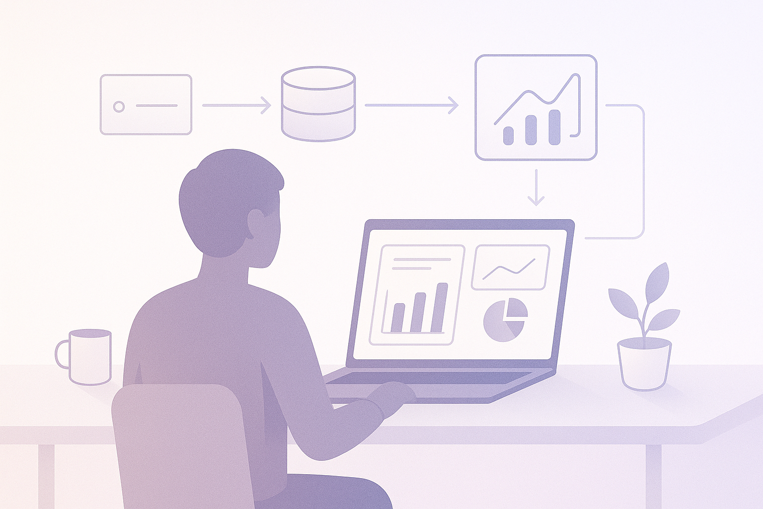
Monthly gateway release posts are usually the corporate equivalent of dry toast. A version number appears. Power BI Desktop compatibility gets a polite bow. Then everyone goes back to moving data and arguing with refresh logs.
The February 2026 on-premises data gateway release is mostly that kind of update. Microsoft says the build is 3000.306, and the point is simple: keep the gateway aligned with the February 2026 Power BI Desktop release so reports refreshed through the gateway use the same query execution logic and runtime as Desktop.
Useful? Yes. Dramatic? Not even a little.
What makes this release worth a Spark team’s time is everything happening around it. In the last few months, Microsoft added manual gateway updates, shipped pipeline performance work in January, and expanded managed private endpoint guidance for Fabric Data Engineering workloads. Put together, those changes tell a clearer story than the February post does on its own: the gateway still matters, but it is no longer background plumbing you patch whenever someone remembers.
The February release itself is small
The official February announcement is short and very Power BI flavored. Version 3000.306 brings the gateway up to date with the February 2026 Power BI Desktop release. That matters if your Spark world touches gateway-mediated refresh or movement of data through Fabric services that depend on the gateway.
If your team uses Spark notebooks or Spark job definitions alongside pipelines, semantic models, or refresh paths that still run through the on-premises data gateway, version alignment is not glamorous, but it is part of keeping production boring. And boring is what you want from production. “Interesting” is how incident reviews begin.
There is also an awkward timing detail here. The Microsoft Learn page for supported gateway versions already lists March 2026, build 3000.310, as the latest supported update. So if you are making an upgrade decision today, the practical move is not to cling to 3000.306 out of loyalty to February. The real lesson from February is that the monthly update train keeps moving, and Spark teams need an operating habit for that cadence.
December changed the maintenance story
The bigger operational shift arrived in the December 2025 release, build 3000.298. That release introduced Manual Update for On-premises Data Gateway in preview. Microsoft says admins can trigger updates from the gateway UI or programmatically through API or script, and the related documentation shows the PowerShell path with Update-DataGatewayClusterMember.
That may sound like a small administrative nicety. It is not. It is the difference between “we update the gateway when someone notices” and “we update the gateway during a planned window, on purpose, with a record of what happened.”
Microsoft’s update documentation is blunt about why this matters in clusters. When gateway members run different versions, you can get sporadic failures because one member can handle a query that another cannot. The guidance is to disable one member, let the work drain, update it, re-enable it, and repeat for the rest of the cluster. That is not fancy advice. It is good advice. Production systems usually break in ordinary, irritating ways.
Two details matter:
The November 2025 release is the baseline for the manual update feature.
Microsoft says the updater service activates only when an update is triggered from the UI or via PowerShell.
In other words, December did not add one more button. It added a more controlled update path for teams that have to care about maintenance windows, change management, and not getting yelled at on a Friday night.
January made the gateway more relevant to pipeline-heavy Spark teams
The January 2026 release, build 3000.302, was modest on paper but more interesting in practice. Microsoft called out two improvements:
Performance optimization for reading CSV format in Copy job and Pipeline activities
Performance optimization for read and write through adaptive performance tuning capability in Pipeline
That is not a fireworks show, but it is more concrete than the average release note. If your Fabric Spark workflow begins with Copy jobs or Pipeline activities that pull CSV-shaped data before Spark takes over, January was the sort of release you should benchmark instead of shrugging at.
Notice what Microsoft did not say: there is no grand promise that everything is suddenly twice as fast and angels now sing over your lakehouse. Fine. Release notes rarely sing. Still, when a gateway sits in front of repetitive ingestion work, even a dull-sounding optimization can shave time off every run. Boring improvements are often the ones that pay rent.
Spark teams now have a second route for on-premises access
The most interesting shift is not in the gateway release notes at all. It is in Fabric’s managed private endpoint work for Data Engineering workloads.
Microsoft’s October 2025 Fabric blog post says Managed Private Endpoints support for connecting to Private Link Services became available through the Fabric Public REST APIs, specifically to help Fabric Spark compute reach on-premises and network-isolated data sources. The newer Learn guidance goes further: Fabric workloads such as Spark or Data Pipelines can connect to on-premises or custom-hosted sources through an approved Private Link setup, with traffic flowing through the Microsoft backbone network rather than the public internet.
That is a real architectural fork in the road.
If your team has treated the on-premises data gateway as the default answer to any sentence containing the words “on-premises” and “Fabric,” that default deserves another look. The managed private endpoint docs say that, once approved, Fabric Data Engineering workloads such as notebooks, Spark job definitions, materialized lakeviews, and Livy endpoints can securely connect to the approved resource.
That does not kill the gateway. It does mean the gateway is no longer the only respectable adult in the room.
There is also one gotcha that will ambush people who like clicking around until things work. Microsoft says creating a managed private endpoint with a fully qualified domain name through Private Link Service is supported only through the REST API, not the UX. So if your plan is “we’ll set it up later in the portal,” later may arrive carrying disappointment.
What a Fabric Spark team should do next
If I were cleaning this up for a real production team, the to-do list would look like this:
Check the supported monthly updates page before touching anything. As of late March 2026, it already lists March 2026, build 3000.310, as the newest supported gateway release.
If you run a gateway cluster, stop tolerating version drift. Follow Microsoft’s member-by-member update guidance so one node does not become the office goblin that fails queries the others can run.
If you want controlled upgrades, confirm your gateways are on the November 2025 baseline or later, then script manual updates with Update-DataGatewayClusterMember.
Inventory which Spark-adjacent workloads really need the gateway and which ones are gateway-shaped only because nobody revisited the design.
For Spark or Data Pipeline scenarios that need private access to on-premises or custom-hosted sources, evaluate managed private endpoints and Private Link Service instead of assuming the gateway must stay in the middle.
If your ingestion path leans on CSV through Copy jobs or Pipeline activities, test the January build improvements against your actual workloads rather than trusting vague optimism.
One more limitation matters here. The managed private endpoint overview says the feature depends on Fabric Data Engineering workload support in both the tenant home region and the capacity region. So before anyone gives a triumphant architecture presentation, check whether your region setup actually supports what you plan to do.
The short version
The February 2026 gateway release is a small compatibility release. On its own, it would barely justify a coffee break. For Fabric Spark teams, though, it lands in the middle of a more meaningful change.
Gateway maintenance is becoming easier to control. Pipeline-oriented gateway work picked up performance tuning in January. And Spark workloads now have a documented private-connectivity path that can bypass the old habit of stuffing every on-premises access pattern through the gateway.
So no, February 2026 was not a blockbuster. It was a signpost. The smart move is to stop treating the gateway as an untouchable default, update it like you mean it, and decide workload by workload whether Spark still needs that middleman.
If you want the raw source material rather than anyone’s interpretation, start here:
Microsoft published a new end-to-end pattern last week. Train a model inside Fabric. Score it against a governed semantic model. Push predictions straight into Power BI. No data exports. No credential juggling.
The blog post walks through a churn-prediction scenario. Semantic Link pulls data from a governed Power BI semantic model. MLflow tracks experiments and registers models. The PREDICT function runs batch inference in Spark. Real-time endpoints serve predictions through Dataflow Gen2. Everything lives in one workspace, one security context, one OneLake.
It reads well. It demos well.
But demo code is not production code. The gap between “it runs in my notebook” and “it runs every Tuesday at 4 AM without paging anyone” is exactly where Fabric Spark teams bleed time.
This is the checklist for crossing that gap.
Prerequisites that actually matter
The official blog assumes a Fabric-enabled workspace and a published semantic model. That is the starting line. Production is a different race.
Capacity planning comes first. Fabric Spark clusters consume capacity units. A batch scoring job running on an F64 during peak BI refresh hours competes for the same CUs your report viewers need. Run scoring in off-peak windows, or provision a separate capacity for data science workloads. Either way, know your CU ceiling before your first experiment. Discovering your scoring job throttles the CFO’s dashboard refresh is not a conversation you want to have.
Workspace isolation is not optional. Dev, test, prod. Semantic models promoted through deployment pipelines. ML experiments pinned to dev. Registered models promoted to prod only after validation passes. If your team trains models in the same workspace where finance runs their quarterly close dashboard, you are one accidental publish away from explaining why the revenue numbers just changed.
MLflow model signatures must be populated from day one. The PREDICT function requires them. No signature, no batch scoring. This constraint is easy to forget during prototyping and expensive to fix later. Make it a rule: every mlflow.sklearn.log_model call includes an infer_signature output. No exceptions. Write a pre-commit hook if you have to.
Semantic Link: the part most teams underestimate
Semantic Link connects your Power BI semantic model to your Spark notebooks. Call fabric.read_table() and you get governed data. Same measures and definitions your business users see in their reports. The data in your model’s training set matches what shows up in Power BI.
This matters more than it sounds.
Every analytics team that has been around long enough has a story about metric inconsistency. “Active customer” means one thing in the DAX model, another thing in the SQL pipeline, and a third thing in the data scientist’s Python notebook. The numbers diverge. Somebody notices. A week of forensic reconciliation follows.
Semantic Link kills that problem at the root. But only if you use it deliberately.
Start with fabric.list_measures(). Audit what DAX measures exist. Understand which ones your model depends on. Then pull data with fabric.read_table() rather than querying lakehouse tables directly. When you need to engineer features beyond what the semantic model provides, document every derivation in a version-controlled notebook. Written down and committed. Not living in someone’s memory or buried in a thread.
Training guardrails worth building
The Fabric blog shows a clean LightGBM training flow with MLflow autologging. That is the happy path. Production needs the unhappy path covered too.
Validate data before training. Check row counts against expected baselines. Check for null spikes in key columns. Check that the class distribution has not shifted beyond your predefined threshold. A model trained on corrupted or stale data produces confident garbage. Confident garbage is worse than no model at all, because people act on it.
Tag every experiment run. MLflow in Fabric supports custom tags. Use them aggressively. Tag each run with the semantic model version it pulled from, the notebook commit hash, and the data snapshot date. Three months from now, when a stakeholder asks why the model flagged 200 customers as high churn risk and zero of them actually left, you need to reconstruct exactly what happened. Without tags, you are guessing.
Build a champion-challenger gate. Before any new model version reaches production, it must beat the current model on a holdout set from the most recent data. Not any holdout set. The most recent one. Automate this comparison in a validation notebook that runs as a pipeline step before model registration. If the challenger fails to clear the margin you defined upfront, the pipeline halts. No override button. No “let’s just push it and see.” The gate exists to prevent optimism from substituting for evidence.
Batch scoring: the PREDICT function in production
Fabric’s PREDICT function is straightforward. Pass a registered MLflow model and a Spark DataFrame. Get predictions back. It supports scikit-learn, LightGBM, XGBoost, CatBoost, ONNX, PyTorch, TensorFlow, Keras, Spark, Statsmodels, and Prophet.
The production requirements are few but absolute.
Write predictions to a delta table in OneLake. Not to a temporary DataFrame that dies with the session. Partition that table by scoring date. Add a column for the model version that generated each row. This is your audit trail. When someone asks “why did customer 4471 show as high risk last Tuesday?”, you pull the partition, check the model version, and have an answer in minutes. Without that structure, the same question costs you a day.
Chain your scoring job to run after your semantic model refresh. Sequence matters. If the model scores data from the prior refresh cycle, your predictions are one step behind reality. Use Fabric pipelines to enforce the dependency explicitly. Refresh completes, scoring starts.
Real-time endpoints: know exactly what you are signing up for
Fabric now offers ML model endpoints in preview. Activate one from the model registry. Fabric spins up managed containers and gives you a REST API. Dataflow Gen2 can call the endpoint during data ingestion, enriching rows with predictions in flight.
The capability is real. The constraints are also real.
Real-time endpoints support a limited set of model flavors: Keras, LightGBM, scikit-learn, XGBoost, and (since January 2026) AutoML-trained models. PyTorch, TensorFlow, and ONNX are not supported for real-time serving. If your production model uses one of those frameworks, batch scoring is your only path.
The auto-sleep feature deserves attention. Endpoints scale capacity to zero after five minutes without traffic. The first request after sleep incurs a cold-start delay while containers spin back up. For use cases that need consistent sub-second latency, you have two options: disable auto-sleep and accept the continuous capacity cost, or send periodic synthetic requests to keep the endpoint warm.
The word “preview” is load-bearing here. Preview means the API can change between updates. Preview means SLAs are limited. Preview means you need a batch-scoring fallback in place before you route any production workflow through a real-time endpoint. Build the fallback first. Test it. Then add the real-time path as an optimization on top.
The rollback plan you need to write before you ship
Most teams build forward. They write the training pipeline, the scoring job, the endpoint, the Power BI report that consumes predictions. Then they ship.
Nobody writes the backward path. Until something goes wrong.
Your rollback plan has three parts.
First, keep at least two prior model versions in the registry. If the current version starts producing bad predictions, you roll back by updating the model alias. One API call. The scoring pipeline picks up the previous version on its next run.
Second, partition prediction tables by date and model version. Rolling back a model means nothing if downstream reports still display the bad predictions. With partitioned tables, you can filter or drop the scoring run from the misbehaving version and revert to the prior run’s output.
Third, a kill switch for real-time endpoints. One API call to deactivate the endpoint. Traffic falls back to the latest batch-scored delta table. Your Power BI report keeps working, just without real-time enrichment, while you figure out what went wrong.
Test this plan. Not on paper. Run the rollback end to end in your dev environment. Time it. If reverting to a stable state takes longer than fifteen minutes, your plan is too complicated. Simplify it until the timer clears.
Ship it
The architecture Microsoft described is sound. Semantic Link for governed data access. MLflow for experiment tracking and model registration. PREDICT for batch scoring to OneLake. Real-time endpoints for low-latency enrichment. Power BI consuming prediction tables through DirectLake or import.
But architecture alone does not keep a system running at 4 AM. The capacity plan does. The workspace isolation does. The data validation gate, the champion-challenger check, the scoring sequence, the endpoint fallback, the rollback drill. Those are what separate a demo from a service.
Do the checklist. Test the failure modes. Then ship.
This post was written with help from anthropic/claude-opus-4-6
Author’s note –I have enjoyed playing around with the Deep Research capabilities of ChatGPT, and I had it put together what it felt was the definitive whitepaper on Capacity Management for Microsoft Fabric. It basically just used the Microsoft documentation (plus a couple of community posts) to pull it together, so I’m curious what you think. I’ll leave a link to download the PDF copy of this at the end of the post.
Executive Summary
Microsoft Fabric capacities provide the foundational compute resources that power the Fabric analytics platform. They are essentially dedicated pools of compute (measured in Capacity Units or CUs) allocated to an organization’s Microsoft Fabric tenant. Proper capacity management is crucial for ensuring reliable performance, supporting all Fabric workloads (Power BI, Data Engineering, Data Science, Real-Time Analytics, etc.), and optimizing costs. This white paper introduces capacity and tenant administrators to the full spectrum of Fabric capacity management – from basic concepts to advanced strategies.
Key takeaways: Fabric offers multiple capacity SKUs (F, P, A, EM, Trial) with differing capabilities and licensing models. Understanding these SKU types and how to provision them is the first step. Once a capacity is in place, administrators must plan and size it appropriately to meet workload demands without over-provisioning. All Fabric experiences share capacity resources, so effective workload management and governance are needed to prevent any one workload from overwhelming others. Fabric’s capacity model introduces bursting and smoothing to handle short-term peaks, while throttling mechanisms protect the system during sustained overloads. Tools like the Fabric Capacity Metrics App provide visibility into utilization and help with monitoring performance and identifying bottlenecks. Administrators should leverage features such as autoscale options (manual or scripted scaling and Spark auto-scaling), notifications, and the new surge protection to manage peak loads and maintain service levels.
Effective capacity management also involves governance practices: assigning workspaces to capacities in a thoughtful way, isolating critical workloads, and controlling who can create or consume capacity resources. Cost optimization is a continuous concern – this paper discusses strategies like pausing capacities during idle periods, choosing the right SKU size (and switching to reserved pricing for savings), and using per-user licensing (Premium Per User) when appropriate to minimize costs. Finally, we present real-world scenarios with recommendations to illustrate how organizations can mix and match these approaches. By following the guidance in this document, new administrators will be equipped to manage Microsoft Fabric capacities confidently and get the most value from their analytics investment.
Introduction to Microsoft Fabric Capacities
Microsoft Fabric is a unified analytics platform that spans data integration, data engineering, data warehousing, data science, real-time analytics, and business intelligence (Power BI). A Microsoft Fabric capacity is a dedicated set of cloud resources (compute memory/CPU) allocated to a tenant to run these analytics workloads. In essence, a capacity represents a chunk of “always-on” compute power measured in Capacity Units (CUs) that your organization owns or subscribes to. The capacity’s size (number of CUs) determines how much computational load it can handle at any given time.
Why capacities matter: Certain Fabric features and collaborative capabilities are only available when content is hosted in a capacity. For example, to share Power BI reports broadly without requiring per-user licenses, or to use advanced Fabric services like Spark notebooks, data warehouses, and real-time analytics, you must use a Fabric capacity. Capacities enable organization-wide sharing, collaboration, and performance guarantees beyond the limits of individual workstations or ad-hoc cloud resources. They act as containers for workspaces – any workspace assigned to a capacity will run all its workload (reports, datasets, pipelines, notebooks, etc.) on that capacity’s resources. This provides predictable performance and isolation: one team’s heavy data science experiment in their capacity won’t consume resources needed by another team’s dashboards on a different capacity. It also simplifies administration – instead of managing separate compute for each project, admins manage pools of capacity that can host many projects.
In summary, Fabric capacities are the backbone of a Fabric deployment, combining compute isolation, performance scaling, and licensing benefits. With a capacity, your organization can create and share Fabric content (from Power BI reports to AI models) with the assurance of dedicated resources and without every user needing a premium license. The rest of this document will explore how to choose the right capacity, configure it for various workloads, keep it running optimally, and do so cost-effectively.
Capacity SKU Types and Differences (F, P, A, EM, Trial)
Microsoft Fabric builds on the legacy of Power BI’s capacity-based licensing, introducing new Fabric (F) SKUs alongside existing Premium (P) and Embedded SKUs. It’s important for admins to understand the types of capacity SKUs available and their differences:
F-SKUs (Fabric SKUs): These are the new* capacity units introduced with Microsoft Fabric. They are purchased through Azure and measured in Capacity Units (CUs). F-SKUs range from small to very large (F2 up to F2048), each providing a set number of CUs (e.g. F2 = 2 CUs, F64 = 64 CUs, etc.). F-SKUs support all Fabric workloads (Power BI content and the new Fabric experiences like Lakehouse, Warehouse, Spark, etc.). They offer flexible cloud purchasing (hourly pay-as-you-go billing with the ability to pause when not in use) and scaling options. Microsoft is encouraging customers to adopt F-SKUs for Fabric due to their flexibility in scaling and billing.
P-SKUs (Power BI Premium per Capacity): These were the traditional Power BI Premium capacities (P1 through P5) bought via the Microsoft 365 admin center with an annual subscription commitment. P-SKUs also support the full Fabric feature set (they have been migrated onto the Fabric backend). However, as of mid-2024, Microsoft has deprecated new purchases of P-SKUs in favor of F-SKUs. Organizations with existing P capacities can use Fabric on them, but new capacity purchases should be F-SKUs going forward. One distinction is that P-SKUs cannot be paused and were billed as fixed annual licenses (less flexible, but previously lower cost for constant use).
A-SKUs (Azure Power BI Embedded): These are Azure-purchased capacities originally meant for Power BI embedded analytics scenarios. They correspond to the same resource levels as some F-SKUs (for example, A4 is equivalent to an F64 in compute power) but only support Power BI workloads – they do not support the new Fabric experiences like Spark or data engineering. A-SKUs can still be used if you only need Power BI (for example, for embedding reports in a web app), but if any Fabric features are needed, you must use an F or P SKU.
EM-SKUs (Power BI Embedded for organization): Another variant of embedded capacity (EM1, EM2, EM3) which are lower-tier and were used for internal “Embedded” scenarios (like embedding Power BI content in SharePoint or Teams without full Premium). Like A-SKUs, EM SKUs are limited to Power BI content only and correspond to smaller capacity sizes (EM3 ~ F32). They cannot run Fabric workloads.
Trial SKU: Microsoft Fabric offers a free trial capacity to let organizations try Fabric for a limited time. The trial capacity provides 64 CUs (equivalent to an F64 SKU) and supports all Fabric features, but lasts for 60 days. This is a fixed-size capacity (roughly equal to a P1 in power) that can be activated without cost. It’s ideal for initial evaluations and proof-of-concept work. After 60 days, the trial expires (though Microsoft has allowed extensions in some cases). Administrators cannot change the size of a trial capacity – it’s pre-set – and there may be limits on the number of trials per tenant.
The table below summarizes the Fabric SKU sizes and their approximate equivalence to Power BI Premium for context:
SKU
Capacity Units (CUs)
Equivalent P-SKU / A-SKU
Power BI v-cores
F2
2 CUs
(no P-SKU; smallest)
0.25 v-core
F4
4 CUs
(no P-SKU)
0.5 v-core
F8
8 CUs
EM1 / A1
1 v-core
F16
16 CUs
EM2 / A2
2 v-cores
F32
32 CUs
EM3 / A3
4 v-cores
F64
64 CUs
P1 / A4
8 v-cores
Trial
64 CUs
(no P-SKU; free trial)
8 v-cores
F128
128 CUs
P2 / A5
16 v-cores
F256
256 CUs
P3 / A6
32 v-cores
F512
512 CUs
P4 / A7
64 v-cores
F1024
1024 CUs
P5 / A8
128 v-cores
F2048
2048 CUs
(no direct P-SKU)
256 v-cores
Table: Fabric capacity SKU sizes in Capacity Units (CU) with equivalent legacy SKUs. Note: P-SKUs P1–P5 correspond to F64–F1024. A-SKUs and EM-SKUs only support Power BI content and roughly map to F8–F32 sizes.
In practical terms, F64 (64 CU) is the threshold where a capacity is considered “Premium” in the Power BI sense – it has the same 8 v-cores as a P1. Indeed, content in workspaces on an F64 or larger can be consumed by viewers with a free Fabric license (no Pro license needed). By contrast, the smaller F2–F32 capacities, while useful for light workloads or development, do not remove the need for Power BI Pro licenses for content consumers. Administrators should be aware of this distinction: if your goal is to enable broad internal report sharing to free users, you will need at least an F64 capacity.
To recap SKU differences: F-SKUs are the modern, Azure-based Fabric capacities that cover all workloads and offer flexibility (pause/resume, hourly billing). P-SKUs (legacy Premium) also cover all workloads but are being phased out for new purchases, and they require an annual subscription (though existing ones can continue to be used for Fabric). A/EM SKUs are limited to Power BI content only and primarily used for embedding scenarios; they might still be relevant if your organization only cares about Power BI and wants a smaller or cost-specific option. And the trial capacity is a temporary F64 equivalent provided free for evaluation purposes.
Licensing and Provisioning
Before you can use a Fabric capacity, you must license and provision it for your tenant. This involves understanding how to acquire the capacity (through Azure or Microsoft 365), what user licenses are needed, and how to set up the capacity in the admin portal.
Purchasing a capacity: For F-SKUs and A/EM SKUs, capacities are purchased via an Azure subscription. You (or your Azure admin) will create a Microsoft Fabric capacity resource in Azure, selecting the SKU size (e.g. F64) and region. The capacity resource is billed to your Azure account. For P-SKUs (if you already have one), they were purchased through the Microsoft 365 admin center (as a SaaS license commitment). As noted, new P-SKU purchases are no longer available after July 2024. If you have existing P capacities, they will show up in the Fabric admin portal automatically. Otherwise, new capacity needs will be fulfilled by creating F-SKUs in Azure.
Provisioning and setup: Once purchased, the capacity must be provisioned in your Fabric tenant. For Azure-based capacities (F, A, EM), this happens automatically when you create the resource – you will see the new capacity listed in the Fabric Admin Portal under Capacity settings. You need to be a Fabric admin or capacity admin to access this. In the Fabric Admin Portal (accessible via the gear icon in the Fabric UI), under Capacity Settings, you will find tabs for Power BI Premium, Power BI Embedded, Fabric capacity, and Trial. Your capacity will appear in the appropriate section (e.g., an F-SKU under “Fabric capacity”). From there, you can manage its settings (more on that later) and assign workspaces to it.
When creating an F capacity in Azure, you will choose a region (datacenter location) for the capacity. This determines where the compute resources live and typically where the data for Fabric items in that capacity is stored. For example, if you create an F64 in West Europe, a Fabric Warehouse or Lakehouse created in a workspace on that capacity will reside in West Europe region (useful for data residency requirements). Organizations with global presence might provision capacities in multiple regions to keep data and computation local to users or comply with regulations.
Per-user licensing requirements: Even with capacities, Microsoft Fabric uses a mix of capacity licensing and per-user licenses:
Every user who authors content or needs access to Power BI features beyond viewing must have a Power BI Pro license (or Premium Per User) unless the content is in a capacity that allows free-user access. In Fabric, a Free user license lets you create and use non-Power BI Fabric items (like Lakehouses, notebooks, etc.) in a capacity workspace, but it does not allow creating standard Power BI content in shared workspaces or sharing those with others. To publish Power BI reports to a workspace (other than your personal My Workspace) and share them, you still need a Pro license or PPU. Essentially, capacity removes license requirements for viewing content (if the capacity is sufficiently large), but content creators typically need Pro/PPU licenses for Power BI work.
For viewers of content: If the workspace is on a capacity smaller than F64, all viewers need Pro licenses as if it were a normal shared workspace. If the workspace is on an F64 or larger capacity (or a P-SKU capacity), then free licensed users can view the content (they just need the basic Fabric free license and viewer role). This is analogous to Power BI Premium capacity behavior. So an admin must plan license needs accordingly – for true wide audience distribution, ensure the capacity is at least F64, otherwise you won’t realize the “free user view” benefit.
Premium Per User (PPU): PPU is a per-user licensing option that provides most Premium features to individual users on shared capacity. While not a capacity, it’s relevant in capacity planning: if you have a small number of users that need premium features, PPU can be more cost-effective than buying a whole capacity. Microsoft suggests considering PPU if fewer than ~250 users need Premium capabilities. For example, rather than an F64 which supports unlimited users, 50 users could each get PPU licenses. However, PPU does not support the broader Fabric workloads (it’s mainly a Power BI feature set license), so if you want the Fabric engineering/science features, you need a capacity.
In summary, to get started you will purchase or activate a capacity and ensure you have at least one user with a Pro (or PPU) license to administer it and publish Power BI content. Many organizations begin with the Fabric trial capacity – any user with admin rights can initiate the trial from the Fabric portal, which creates the 60-day F64 capacity for the tenant. During the trial period, you might allow multiple users to experiment on that capacity. Once ready to move to production, you would purchase an F-SKU of appropriate size. Keep in mind that a trial capacity is time-bound and also fixed in size (you cannot scale a trial up or down). So after gauging usage in trial, you’ll choose a permanent SKU.
Capacity Planning and Sizing Guidance
Choosing the right capacity size is a critical early decision. Capacity planning is the process of estimating how many CUs (or what SKU tier) you need to run your workloads smoothly, both now and in the future. The goal is to avoid performance problems like slow queries or job failures due to insufficient resources, while also not over-paying for idle capacity. This section provides guidance on sizing a capacity and adjusting it as usage evolves.
Understand your workloads and users: Start by profiling the types of workloads and usage patterns you expect on the capacity. Key factors include:
Data volume and complexity: Large data models (e.g. huge Power BI datasets) or heavy ETL processes (like frequent dataflows or Spark jobs) will consume more compute and memory. If you plan to refresh terabyte-scale datasets or run complex transformations daily, size up accordingly.
Concurrent users and activities:Power BI workloads with many simultaneous report users or queries (or heavy embedded analytics usage) can drive up CPU and memory usage quickly. A capacity serving 200 concurrent dashboard users needs more CUs than one serving 20 users. Concurrency in Spark jobs or SQL queries similarly affects load.
Real-time or continuous processing: If you have real-time analytics (such as continuous event ingestion, KQL databases for IoT telemetry, or streaming datasets), your capacity will see constant usage rather than brief spikes. Ongoing processes mean you need enough capacity to sustain a baseline of usage 24/7.
Advanced analytics and data science:Machine learning model training or large-scale data science experiments can be very computationally intensive (high CPU for extended periods). A few data scientists running complex notebooks might consume more CUs than dozens of basic report users. Also consider if they will run jobs concurrently.
Number of users/roles: The more users with access, the greater the chance of overlapping activities. A company with 200 Power BI users running reports will likely require more capacity than one with 10 engineers doing data transformations. Even if each individual task isn’t huge, many small tasks add up.
By evaluating these factors, you can get a rough sense of whether you need a small (F2–F16), medium (F32–F64), or large (F128+) capacity.
Start with data and tools: Microsoft recommends a data-driven approach to capacity sizing. One strategy is to begin with a trial capacity or a small pay-as-you-go capacity, run your actual workloads, and measure the utilization. The Fabric Capacity Metrics App can be installed to monitor CPU utilization, memory, etc., and identify peaks. Over a representative period (say a busy week), observe how much of the 64 CU trial is used. If you find that utilization is peaking near 100% and throttling occurs, you likely need a larger SKU. If usage stays low (e.g. under 30% most of the time), you might get by with a smaller SKU in production or keep the same size with headroom.
Microsoft provides guidance to “start small and then gradually increase the size as necessary.” It’s often best to begin with a smaller capacity, see how it performs, and scale up if you approach limits. This avoids overcommitting to an expensive capacity that you might not fully use. With Fabric’s flexibility, scaling up (or down) capacity is relatively easy through Azure, and short-term overuse can be mitigated by bursting (discussed later).
Concretely, you would:
Measure consumption – perhaps use an F32 or F64 on a trial or month-to-month basis. Use the metrics app to check the CU utilization over time (Fabric measures consumption in 30-second intervals; multiply CUs by 30 to get CU-seconds per interval). Identify peak times and which workloads are driving them (the metrics app breaks down usage by item type, e.g. dataset vs Spark notebook).
Identify requirements – If your peak 30-second CU use is, say, 1500 CU-seconds, that’s roughly 50 CUs worth of power needed continuously in that peak period (since 30 sec * 50 CU = 1500). That suggests an F64 might be just enough (64 CUs) with some buffer, whereas an F32 (32 CUs) would throttle. On the other hand, if peaks only hit 200 CU-seconds (which is ~7 CUs needed), even an F8 could handle it.
Scale accordingly – Choose the SKU that covers your typical peak. It’s wise to allow some headroom, as constant 100% usage will lead to throttling. For instance, if your trial F64 shows occasional 80% spikes, moving to a permanent F64 could be fine thanks to bursting, but if you often hit 120%+ (bursting into future capacity), you should consider F128 or splitting workloads.
Microsoft has also provided a Fabric Capacity Estimator tool (on the Fabric website) which can help model capacity needs by inputting factors like number of users, dataset sizes, refresh rates, etc. This can be a starting point, but real usage metrics are more reliable.
Planning for growth and variability: Keep in mind future growth – if you expect user counts or data volumes to double in a year, factor that into capacity sizing (you may start at F64 and plan to increase to F128 later). Also consider workload timing. Some capacities experience distinct daily peaks (e.g., heavy ETL jobs at 2 AM, heavy report usage at 9 AM). Thanks to Fabric’s bursting and smoothing, a capacity can handle short peaks above its baseline, but if two peaks overlap or usage grows, you might need a bigger size or to schedule workloads to avoid contention. Where possible, schedule intensive background jobs (data refreshes, scoring runs) during off-peak hours for interactive use, to reduce concurrent strain on the capacity.
In summary, do your homework with a trial or pilot phase, leverage monitoring tools, and err on the side of starting a bit smaller – you can always scale up. Capacity planning helps you choose the right SKU and avoid slow queries or throttling while optimizing spend. And remember, you can have multiple capacities too; sometimes the answer is not one gigantic capacity, but two or three medium ones splitting different workloads (we’ll discuss this in governance).
Workload Management Across Fabric Experiences
One of the powerful aspects of Microsoft Fabric is that a single capacity can run a diverse set of workloads: Power BI reports, Spark notebooks, data pipelines, real-time KQL databases, AI models, etc. The capacity’s compute is shared by all these workloads. This section explains how to manage and balance different workloads on a capacity.
Unified capacity, multiple workloads: Fabric capacities are multi-tenant across workloads by design – you don’t buy separate capacity for Power BI vs Spark vs SQL. For example, an F64 capacity could simultaneously be handling a Power BI dataset refresh, a SQL warehouse query, and a Spark notebook execution. All consume from the same pool of 64 CUs. This unified model simplifies architecture: “It doesn’t matter if one user is using a Lakehouse, another is running notebooks, and a third is executing SQL – they can all share the same capacity.” All items in workspaces assigned to that capacity draw on its resources.
However, as an admin, you need to be mindful of resource contention: a very heavy job of one type can impact others. Fabric tries to manage this with an intelligent scheduler and the bursting/smoothing mechanism (which prioritizes interactive operations). Still, you should consider the nature of workloads when assigning them to capacities. Some guidance:
Power BI workloads: These include interactive report queries (DAX queries against datasets), dataset refreshes, dataflows, AI visuals, and paginated reports. In the capacity settings, admins have specific Power BI workload settings (for example, enabling the AI workload for cognitive services, or adjusting memory limits for datasets, similar to Power BI Premium settings). Ensure these are configured as needed – e.g., if you plan on using AI visualizations or AutoML in Power BI, make sure the AI workload is enabled on the capacity. Large semantic models (datasets) can consume a lot of memory; by default Fabric will manage their loading and eviction, but you may want to keep an eye on total model sizes relative to capacity. Paginated reports can be enabled if needed (they can be memory/CPU heavy during execution).
Data Engineering & Science (Spark): Fabric provides Spark engines for notebooks and job definitions. By default, when a Spark job runs, it uses a portion of the capacity’s cores. In fact, for Spark workloads, Microsoft has defined that each 1 CU = 2 Spark vCores of compute power. For example, an F32 (32 CU) capacity has 64 Spark vCores available to allocate across Spark clusters. These vCores are dynamically allocated to Spark sessions as users run notebooks or Spark jobs. Spark has a built-in concurrency limit per capacity: if all Spark vCores are in use, additional Spark jobs will queue until resources free up. As an admin, you can allow or disallow workspace admins from configuring Spark pool sizes on your capacity. If you enable it, power users might spin up large Spark executors that use many cores – beneficial for performance, but potentially starving other workloads. If Spark usage is causing contention, consider limiting the max Spark nodes or advising users to use moderate sizes. Notably, Fabric capacities support bursting for Spark as well – the system can utilize up to 3× the purchased Spark vCores temporarily to run more Spark tasks in parallel. This helps if you occasionally have many Spark jobs at once, but sustained overuse will still queue or throttle. For heavy Spark/ETL scenarios, you might dedicate a capacity just for that to isolate it from BI users.
Data Warehousing (SQL) and Real-Time Analytics (KQL): These workloads run SQL queries or KQL (Kusto Query Language) queries against data warehouses or real-time analytics databases. They consume CPU during query execution and memory for caching data. They are treated as background jobs if run via scheduled processes, or interactive if triggered by a user query. Fabric’s smoothing generally spreads out heavy background query loads over time. Nevertheless, a very expensive SQL query can momentarily spike CPU. As admin, ensure your capacity can handle peak query loads or advise your data teams to optimize queries (like proper indexing on warehouses) to avoid excessive load. There are not many specific toggles for SQL/KQL workloads in capacity settings (beyond enabling the Warehouse or Real-Time Analytics features which are on by default for F and P capacities).
OneLake and data movement: OneLake is the storage foundation for Fabric. While data storage itself doesn’t “consume” capacity CPU (storage is separate), activities like moving data (copying via pipelines), scanning large files, or loading data into a dataframe will use capacity compute. Data integration pipelines (if using Data Factory in Fabric) also run on the capacity. Keep an eye on any heavy data copy or transformation activities, as those are background tasks that could contribute to load.
Isolation and splitting workloads: If you find that certain workloads dominate the capacity, you might consider splitting them onto separate capacities. For instance, a common approach is to separate “self-service BI” and “data engineering” onto different capacities so that a big Spark job doesn’t slow down a business report refresh. Microsoft notes that provisioning multiple capacities can isolate compute for high-priority items or different usage patterns. You could have one capacity dedicated to Power BI content for executives (ensuring their reports are always snappy), and a second capacity for experimental data science projects. This kind of workload isolation via capacities is a governance decision (we will cover more in the governance section). The trade-off is cost and utilization – separate capacities ensure no interference, but you might end up with unused capacity in each if peaks happen at different times. A single capacity shared by all can be more cost-efficient if the workloads’ peak times are complementary.
Tenant settings delegation: In Fabric, some tenant-level settings (for example, certain Power BI tenant settings or workload features) can be delegated to the capacity level. This means you can override a global setting for a specific capacity. For instance, you might have a tenant setting that limits the maximum size of Power BI datasets for Pro workspaces, but for a capacity designated to a specific team, you allow larger models. In the capacity management settings, check the Delegated tenant settings section if you need to tweak such options for one capacity without affecting others. This feature allows granular control, such as enabling preview features or higher limits on a capacity used by advanced users while keeping defaults elsewhere.
Monitoring workload mix: Use the Capacity Metrics App or the Fabric Monitoring Hub to see what types of operations are consuming the most resources. The app can break down usage by item type (e.g., dataset vs Spark vs pipeline) to help identify if one category is the culprit for high utilization. If you notice, for example, that Spark jobs are consistently using the majority of CUs (perhaps visible as high background CPU), it may prompt you to adjust Spark configurations or move some Spark-heavy workspaces off to another capacity.
In summary, Fabric capacities are shared across all workload types, which is great for flexibility but requires good management to ensure balance. Leverage capacity settings to tune specific workloads (Power BI workload enabling, Spark pool limits, etc.), monitor the usage by workload type, and consider logical separation of workloads via multiple capacities if needed. Microsoft Fabric is designed so that the platform itself handles a lot of the balancing (through smoothing of background jobs), but administrator insight and control remain important to avoid any single workload overwhelming the rest.
Isolation and Security Boundaries
Microsoft Fabric capacities play a role in isolation at several levels – performance isolation, security isolation, and even geographic isolation. It’s important to understand what a capacity isolates (and what it doesn’t) within a Fabric tenant, and how to leverage capacities for governance or compliance.
Performance and resource isolation: A capacity is a unit of isolation for compute resources. Compute usage on one capacity does not affect other capacities in the tenant. If Capacity A is overloaded and throttling, it will not directly slow down Capacity B, since each has its own quota of CUs and separate throttling counters. This means you can confidently separate critical workloads by placing them in different capacities to ensure that heavy usage in one area (e.g., a dev/test environment) cannot degrade the performance of another (e.g., production reports). The Fabric platform applies throttling at the capacity scope, so even within the same tenant, one capacity “failing” (hitting limits) doesn’t spill over into another. As noted, there is an exception when it comes to cross-capacity data access: if a Fabric item in Capacity B is trying to query data that resides in Capacity A (for example, a dataset in B accessing a Lakehouse in A via OneLake), then the consuming capacity’s state is what matters for throttling that query. Generally, such cross-capacity consumption is not common except through shared storage like OneLake, and the compute to actually retrieve the data will be accounted to the consumer’s capacity.
Security and content isolation: It’s crucial to realize that a capacity is not a security boundary in terms of data access. All Fabric content security is governed by Entra ID (Azure AD) identities, roles, and workspace permissions, not by capacity. For example, just because Workspace X is on Capacity A and Workspace Y is on Capacity B does not mean users of X cannot access Y – if a user has the right permissions, they can access both. Capacities do not define who can see data; they define where it runs. So if you have sensitive data that only certain users should access, you still must rely on workspace-level security or separate Entra tenants, not merely separate capacities.
That said, capacities can assist with administrative isolation. You can delegate capacity admin roles so that different people manage different capacities. For instance, the finance IT team might be given admin rights to the “Finance Capacity” and they can control which workspaces go into it, without affecting other capacities. Additionally, you can control which workspaces are assigned to which capacity. By limiting capacity assignment rights (via the Contributor permissions setting on a capacity, which you can restrict to specific security groups), you ensure that, say, only approved workspaces/projects go into a certain capacity. This can be thought of as a soft isolation: e.g., only the HR team’s workspaces are placed in the HR capacity, keeping that compute “clean” from others.
Geographical and compliance isolation: If your organization has data residency requirements (for example, EU data must stay in EU datacenters, US data in US), capacities are a useful construct. When you create a capacity, you choose an Azure region for it. Workspaces on that capacity will allocate their Fabric resources in that region. This means you can satisfy multi-geo requirements by having separate capacities in each needed region and assigning workspaces accordingly. It isolates the data and compute to that geography. (Do note that OneLake has a global aspect, but it stores files/objects in the region of the capacity or the region you designate when creating the item. Check Fabric documentation on multi-geo support for details – company examples show deploying capacities per geography).
Tenant isolation: The ultimate isolation boundary is the Microsoft Entra tenant. Fabric capacities exist within a tenant. If you truly need completely separate environments (different user directories, no possibility of data or admin overlap), you would use separate Entra tenants (as was illustrated by Microsoft with one company using two tenants for different divisions). That, however, is a very high level of isolation usually only used in scenarios like M&A, extreme security separation, or multi-tenant services. Within one tenant, capacities give you isolation of compute but not identity.
Network isolation: As a side note, Fabric is a cloud SaaS, but it does provide features like Managed Virtual Networks for certain services (e.g., Data Factory pipelines or Synapse integration). These features allow you to restrict outbound data access to approved networks. While not directly related to capacity, these network security options can be enabled per workspace or capacity environment to ensure data does not leak to the public internet. If your organization requires network isolation, investigate Fabric’s managed VNet and private link support for the relevant workloads.
In summary, use capacities to create performance and administrative isolation within your tenant. Assign sensitive or mission-critical workloads their own capacity so they are shielded from others’ activity. But remember that all capacities under a tenant still share the same identity and security context; manage access via roles and perhaps use separate tenants if absolute isolation is needed. Also use capacities for geo-separation if needed by creating them in the appropriate regions.
Monitoring and Metrics
Continuous monitoring of capacity health and usage is vital to ensure you are getting the most out of your capacity and to preempt any issues like throttling. Microsoft Fabric provides several tools and metrics for capacity and workload monitoring.
Capacity Utilization Metrics: The primary tool for capacity admins is the Fabric Capacity Metrics App. This is a Power BI app (or report template) provided by Microsoft that connects to your capacity’s telemetry. It offers dashboards showing CPU utilization (%) over time, broken down by workloads and item types. You can see, for example, how much CPU was used by Spark vs datasets vs queries, etc., and identify the top consuming activities. The app typically looks at recent usage (last 7 days or 30 days) in 30-second intervals. Key visuals include the Utilization chart (showing how close to capacity limit you are) and possibly specific charts for interactive vs background load. As an admin, you should regularly review these metrics. Spikes to 100% indicate that you’re using all available CUs and likely bursting beyond capacity (which could lead to throttling if sustained). If you notice consistent high usage, it may be time to optimize or scale up.
Throttling indicators: Monitoring helps reveal if throttling is occurring. In Fabric, throttling can manifest as delays or failures of operations when the capacity is overextended. The metrics app might show when throttling events happen (e.g., a drop in throughput or specific events count). Additionally, some signals of throttling include user reports of slowness, refresh jobs taking longer or failing with capacity errors, or explicit error messages. Fabric may return an HTTP 429 or 430 error for certain overloaded scenarios (for example, Spark jobs will give a specific error code 430 if capacity is at max concurrency). As admin, watch for these in logs or user feedback.
Real-time monitoring: For current activity, the Monitoring Hub in the Fabric portal provides a view of running and recent operations across the tenant. You can filter by capacity to see what queries, refreshes, Spark jobs, etc., are happening “now” on a capacity and their status. This is useful if the capacity is suddenly slow – you can quickly check if a particular job is consuming a lot of resources. The Monitoring Hub will show active operations and those queued or delayed due to capacity.
Administrator Monitoring Workspace: Microsoft has an Admin Monitoring workspace (sometimes automatically available in the tenant or downloadable) that contains some pre-built reports showing usage and adoption metrics. This might include things like the most active workspaces, most refreshed datasets, etc., across capacities. It’s more about usage analytics, but it can help identify which teams or projects are heavily using the capacity.
External monitoring (Log Analytics): For more advanced needs, you can connect Fabric (especially Power BI aspects) to Azure Log Analytics to capture certain logs, and also collect logs from the On-premises Data Gateway (if you use one). Log Analytics might collect events like dataset refresh timings, query durations, etc. While not giving direct CPU usage, these can help correlate if failures coincide with high load times.
Key metrics to watch:
CPU Utilization %: How close to max CUs you are over time. Spikes to 100% sustained for multiple minutes are a red flag.
Memory: Particularly for Power BI (dataset memory consumption) – if you load multiple large models, ensure they fit in memory. The capacity metrics app shows memory usage per dataset. If near the limits, consider larger capacity or offloading seldom-used models.
Active operations count: Many concurrent operations (queries, jobs) can hint at saturation. For instance, if dozens of queries run simultaneously, you might hit limits even if each is light.
Throttle events: If the metrics indicate delayed or dropped operations, or the Fabric admin portal shows notifications of throttling, that’s a clear indicator.
Notifications: A best practice is to set up alerts/notifications when capacity usage is high. The Fabric capacity settings allow you to configure email notifications if utilization exceeds a certain threshold for a certain time. For example, you might set a notification if CPU stays over 80% for more than 5 minutes. This proactive alert can prompt you to intervene (perhaps scale up capacity or investigate the cause) before users notice major slowdowns.
SLA and user experience: Ultimately, the reason we monitor is to ensure a good user experience. Identify patterns like time of day spikes (maybe every Monday 9AM there’s a huge hit) and mitigate them (maybe by rescheduling some background tasks). Also track the performance of key reports or jobs over time – if they start slowing down, it could be capacity pressure.
In summary, leverage the available telemetry: Fabric Capacity Metrics App for historical trends, Monitoring Hub for real-time oversight, and set up alerts. By keeping a close eye on capacity metrics, you can catch issues early (such as creeping utilization that approaches limits) and take action – whether optimization, scaling, or spreading out the workload – to maintain smooth operations.
Autoscale and Bursting: Managing Peak Loads
One of the novel features of Microsoft Fabric’s capacity model is how it handles peak demands through bursting and smoothing, effectively providing an “autoscaling” experience within the capacity. In this section, we explain these concepts and how to plan for bursts, as well as other autoscale options (such as manual scale-out and Spark autoscaling).
Bursting and smoothing: Fabric is designed to deliver fast performance, even for short spikes in workload, without requiring you to permanently allocate capacity for the peak. It does this via bursting, which allows the capacity to temporarily use more compute than its provisioned CU limit when needed. In other words, your capacity can “burst” above 100% utilization for a short period so that intensive operations finish quickly. This is complemented by smoothing, which is the system’s way of averaging out that burst usage over time so that you’re not immediately penalized. Smoothing spreads the accounting of the consumed CUs over a longer window (5 minutes for interactive operations, up to 24 hours for background operations).
Put simply: “Bursting lets you use more power than you purchased (within a specific timeframe), and smoothing makes sure this over-use is under control by spreading its impact over time.”. For example, if you have an F64 capacity but a particular query needs the equivalent of 128 CUs for a few seconds, Fabric will allow it – the job will complete faster thanks to bursting beyond 64 CUs. Then, the “excess” usage is smoothed into subsequent minutes (meaning for some time after, the capacity’s available headroom is reduced as it pays back that borrowed compute). This mechanism gives an effect similar to short-term autoscaling: the capacity behaves as if it scaled itself up to handle a bursty load, then returns to normal.
Throttling and limits: Bursting is not infinite – it’s constrained by how much future capacity you can borrow via smoothing. Fabric has a throttling policy that kicks in if bursts go on too long or too high. The system tolerates using up to 10 minutes of future capacity with no throttling (this is like a built-in grace period). If you consume more than 10 minutes worth of CUs in advance, Fabric will start applying gentle throttling: interactive operations get a small 20-second delay on submission when between 10 and 60 minutes of capacity overage is consumed. This is phase 1 throttling – users might notice a slight delay but operations still run. If the capacity has consumed over an hour of future CUs (meaning it’s been running well above its quota for a sustained period), it enters phase 2 where interactive operations are rejected outright (while background jobs can still start). Finally, if over 24 hours of capacity is consumed (an extreme overload), all operations (interactive and background) are rejected until usage recovers. The table below summarizes these stages:
Excess Usage (beyond capacity)
System Behavior
Impact
Up to 10 minutes of future capacity
Overage protection (bursting)
No throttling; operations run normally.
10 – 60 minutes of overuse
Interactive delay
New interactive operations (user queries, etc.) are delayed ~20s in queue. Background jobs still start immediately.
60 minutes – 24 hours of overuse
Interactive rejection
New interactive operations are rejected (fail immediately). Background jobs continue to run/queue.
Over 24 hours of overuse
Full rejection
All new operations are rejected (both interactive and background) until the capacity “catches up”.
Table: Throttling thresholds in Fabric’s capacity model. Fabric bursts up to 10 minutes with no penalty. Beyond that, throttling escalates in stages to protect the system.
For most well-managed capacities, you ideally operate in the safe zone (under 10 minutes overage) most of the time. Occasional dips into the 10-60 minute range are fine (users might not even notice the minor delays). If you ever hit the 60+ minute range, that’s a sign the capacity is under-provisioned for the workload or a particular job is too heavy – it should prompt optimization or scaling.
Autoscaling options: Unlike some cloud services that spin up new instances automatically, Fabric’s approach to autoscale is primarily through bursting (which is automatic but time-limited). However, you do have some manual or semi-automatic options:
Manual scale-up/down: Because F-SKUs are purchased via Azure, you can scale the capacity resource to a different SKU on the fly (e.g., from F64 to F128 for a day, then back down). If you have a reserved base (like an F64 reserved instance), you can temporarily scale up using pay-as-you-go to a larger SKU to handle a surge. For instance, an admin might anticipate heavy year-end processing and raise the capacity for that week. Microsoft will bill the overage at the hourly rate for the higher SKU during that period. This is a proactive autoscale you perform as needed. It’s not automatic, but you could script it or use Azure Automation/Logic Apps to trigger scaling based on metrics (there are solutions shared by the community to do exactly this).
Scale-out via additional capacity: Another approach if facing continual heavy load is to add another capacity and redistribute work. For example, if one capacity is maxed out daily, you could purchase a second capacity and move some workspaces to it (spreading the load). This isn’t “autoscale” per se (since it’s a static split unless you later combine them), but it’s a way to increase total resources. Because Fabric charges by capacity usage, two F64s cost the same as one F128 in pay-go terms, so cost isn’t a downside, and you gain isolation benefits.
Spark autoscaling within capacity: For Spark jobs, Fabric allows configuration of auto-scaling Spark pools (the number of executors can scale between a min and max) which optimizes resource usage for Spark jobs. This feature, however, operates within the capacity’s limits – it won’t exceed the total cores available unless bursting provides headroom. It simply means a Spark job will request more nodes if needed and free them when done, up to what the capacity can supply. There is also a preview feature called Spark Autoscale Billing which, if enabled, can offload Spark jobs to a completely separate serverless pool billed independently. That effectively bypasses the capacity for Spark (useful if you don’t want Spark competing with your capacity at all), but since it’s a preview and separate billing, most admins will primarily consider it if Spark is a huge part of their usage and they want a truly elastic experience.
Surge Protection: Microsoft introduced surge protection (currently in preview) for Fabric capacities, which is a setting that limits the total amount of background compute that can run when the capacity is under strain. If enabled, when interactive activities surge, the system will start rejecting background jobs preemptively so that interactive users aren’t as affected. This doesn’t give more capacity, but it triages usage to favor user-driven queries. It’s a protective throttle that helps the capacity recover faster from a spike. As an admin, if you have critical interactive workloads, you might turn this on to ensure responsiveness (at the cost of some background tasks failing and needing retry).
Clearing overuse: If your capacity does get into a heavily throttled state (e.g., many hours of overuse accumulated), one way to reset is to pause and resume the capacity. Pausing essentially stops the capacity (dropping all running tasks) and when resumed, it starts fresh with no prior overhang – but note, any un-smoothed burst usage gets immediately charged at that point. In effect, pausing is like paying off your debt instantly (since when the capacity is off, you can’t “pay back” with idle time, so you are billed for the overage). This is a drastic action (users will be disrupted by a pause), so it’s not a routine solution, but in extreme cases an admin might do this during off hours to clear a badly throttled capacity. Typically, optimizing the workload or scaling out is preferable to hitting this situation.
Design for bursts: Thanks to bursting, you don’t have to size your capacity for the absolute peak if it’s short-lived. Plan for the daily average or slightly above instead of the worst-case peak. Bursting will handle the occasional spike that is, say, 2-3× your normal usage for a few minutes. For example, if your daily work typically uses ~50 CUs but a big refresh at noon spikes to 150 CUs for 1 minute, an F64 capacity can still handle it by bursting (150/64 = ~2.3x for one minute, which smoothing can cover over the next several minutes). This saves cost because you avoid buying an F128 just for that one minute. The system’s smoothing will amortize that one minute over the next 5-10 minutes of capacity. However, if those spikes start lasting 30 minutes or happening every hour, then you do effectively need a larger capacity or you’ll degrade performance.
In conclusion, Fabric’s bursting and smoothing provide a built-in cushion for peaks, acting as an automatic short-term autoscale. As an admin, you should still keep an eye on how often and how deeply you burst (via metrics), and use true scaling strategies (manual scale-up or adding capacity) if needed for sustained load. Also take advantage of features like Spark pool autoscaling and surge protection to further tailor how your capacity handles variable workloads. The combination of these tools ensures you can maintain performance without over-provisioning for rare peaks, achieving a cost-effective balance.
Governance and Best Practices for Capacity Assignment
Managing capacities is not just about the hardware and metrics – it also involves governance: deciding how capacities are used within your organization, which workspaces go where, and enforcing policies to ensure efficient and secure usage. Here are best practices and guidelines for capacity and tenant admins when assigning and governing capacities.
1. Organize capacities by function, priority, or domain: It often makes sense to allocate different capacities for different purposes. For example, you might have a capacity dedicated to production BI content (high priority reports for executives) and another for self-service and development work. This way, heavy experimentation in the dev capacity cannot interfere with the polished dashboards in prod. Microsoft gives an example of using separate capacities so that executives’ reports live on their own capacity for guaranteed performance. Some common splits are:
By department or business unit: e.g., Finance has a capacity, Marketing has another – helpful if departments have very different usage patterns or need cost accountability.
By workload type: e.g., one capacity for all Power BI reports, another for data engineering pipelines and science projects. This can minimize cross-workload contention.
By environment: e.g., one for Production, one for Test/QA, one for Development. This aligns with software lifecycle management.
By geography: as discussed, capacities by region (EMEA vs Americas, etc.) if data residency or local performance is needed.
Having multiple capacities incurs overhead (you must monitor and manage each), so don’t over-segment without reason. But a thoughtful breakdown can improve both performance isolation and clarity in who “owns” the capacity usage.
2. Control workspace assignments: Not every workspace needs to be on a dedicated capacity. Some content can live in the shared (free) capacity if it doesn’t need premium features. As an admin, you should have a process for requesting capacity assignment. You might require that a workspace meet certain criteria (e.g., it’s for a project that requires larger dataset sizes or will have broad distribution) before assigning it to the premium capacity. This prevents trivial or personal projects from consuming expensive capacity resources. In Fabric, you can restrict the ability to assign a workspace to a capacity by using Capacity Contributor permissions. By default, it might allow the whole organization, but you can switch it to specific users or groups. A best practice is to designate a few power users or a governance board that can add workspaces to the capacity, rather than leaving it open to all.
Also consider using the “Preferred capacity for My workspace” setting carefully. Fabric allows you to route user personal workspaces (My Workspaces) to a capacity. While this could utilize capacity for personal analyses, it can also easily overwhelm a capacity if many users start doing heavy work in their My Workspace. Many organizations leave My Workspaces on shared capacity (which requires those users to have Pro licenses for any Power BI content in them) and only put team or app workspaces on the Fabric capacities.
3. Enforce capacity governance policies: There may be tenant-level settings you want to enforce or loosen per capacity. For instance, perhaps in a special capacity for data science you allow higher memory per dataset or allow custom Visualizations that are otherwise disabled. Use the delegated tenant settings feature to override settings on specific capacities as needed. Another example: you might want to disable certain preview features or enforce specific data export rules in a production capacity for security, while allowing them in a dev capacity.
4. Educate workspace owners: Ensure that those who have their workspace on a capacity know the “dos and don’ts.” They should understand that it’s a shared resource – e.g., a badly written query or an extremely large dataset refresh can impact others. Encourage best practices like scheduling heavy refreshes during off-peak times, enabling incremental refresh for large datasets (to reduce refresh load), optimizing DAX and SQL queries, and so on. Capacity admins can provide guidelines or even help review content that will reside on the capacity.
5. Leverage monitoring for governance: Keep track of which workspaces or projects are consuming the most capacity. If one workspace is monopolizing resources (you can see this in metrics, which identify top items), you might decide to move that workspace to its own capacity or address the inefficiencies. You can even implement an internal chargeback or at least show departments how much capacity they consumed to promote accountability.
6. Plan for lifecycle and scaling: Governance also means planning how to scale or reassign as needs change. If a particular capacity is consistently at high load due to growth of a project, have a strategy to either scale that capacity or redistribute workspaces. For example, you might spin up a new capacity and migrate some workspaces to it (admins can change a workspace’s capacity assignment easily in the portal). Microsoft notes you can “scale out” by moving workspaces to spread workload, which is essentially a governance action as much as a performance one. Also, when projects are retired or become inactive, don’t forget to remove their workspaces from capacity (or even delete them) so they don’t unknowingly consume resources with forgotten scheduled operations.
7. Security considerations: While capacity doesn’t enforce security, you can use capacity assignment as part of a trust boundary in some cases. For instance, if you have a workspace with highly sensitive data, you might decide it should run on a capacity that only that team’s admins control (to reduce even the perception of others possibly affecting it). Also, if needed, capacities can be tied to different encryption keys (Power BI allows BYOK for Premium capacities) – check if Fabric supports BYOK per capacity if that’s a requirement.
8. Documentation and communication: Treat your capacities as critical infrastructure. Document which workspaces are on which capacity, what the capacity sizes are, and any rules associated with them. Communicate to your user community about how to request space on a capacity, what the expectations are (like “if you are on the shared capacity, you get only Pro features; if you need Fabric features, request placement on an F SKU” or vice versa). Clear guidelines will reduce ad-hoc and potentially improper use of the capacities.
In essence, governing capacities is about balancing freedom and control. You want teams to benefit from the power of capacities, but with oversight to ensure no one abuses or unknowingly harms the shared environment. Using multiple capacities for natural boundaries (dept, env, workload) and controlling assignments are key techniques. As a best practice, start somewhat centralized (maybe one capacity for the whole org in Fabric’s early days) and then segment as you identify clear needs to do so (such as a particular group needing isolation or a certain region needing its own). This way you keep things manageable and only introduce complexity when justified.
Cost Optimization Strategies
Managing cost is a major part of capacity administration, since dedicated capacity represents a significant investment. Fortunately, Microsoft Fabric offers several ways to optimize costs while meeting performance needs. Here are strategies to consider:
1. Use Pay-as-you-go wisely (pause when idle): F-SKUs on Azure are billed on a per-second basis (with a 1-minute minimum) whenever the capacity is running. This means if you don’t need the capacity 24/7, you can pause it to stop charges. For example, if your analytics workloads are mostly 9am-5pm on weekdays, you could script the capacity to pause at night and on weekends. You only pay for the hours it’s actually on. An F8 capacity left running 24/7 costs roughly $1,200 per month, but if you paused it outside of an 8-hour workday, the cost could drop to a third of that (plus no charge on weekends). Always assess your usage patterns – some organizations run critical reports around the clock, but many could save by pausing during predictable downtime. The Fabric admin portal allows pause/resume, and Azure Automation or Logic Apps can schedule it. Just ensure no important refresh or user query is expected during the paused window.
2. Right-size the SKU (avoid over-provisioning): It might be tempting to get a very large capacity “just in case,” but unused capacity is money wasted. Thanks to bursting, you can usually size for slightly above your average load, not the absolute peak. Monitor utilization and if you see your capacity is consistently under 30% utilized, that’s a sign you might scale down to a smaller SKU and save costs (unless you’re expecting growth or deliberately keeping headroom). The granular SKU options (F2, F4, F8, etc.) let you fine-tune. For instance, if F64 is too much and F32 occasionally struggles, an F48 would be ideal – while not an official SKU, you could achieve an “F48” by using reserved capacity units (more on that below) to split or by alternating scheduling (though that’s complex). Generally, stick to SKUs but choose the lowest one that meets requirements with maybe some buffer.
3. Reserved capacity (annual commitment) for lower rates: Pay-as-you-go is flexible but at a higher unit price. Microsoft has indicated and demonstrated that reserved instance pricing for F-SKUs brings significant cost savings (on the order of ~40% cheaper for a 1-year commitment). For example, an F8 costs around €1188/month pay-go, but ~€706/month with a 1-year reservation. If you know you will need a capacity continuously for a long period, consider switching to a reserved model to reduce cost. Importantly, when you reserve, you are reserving a certain number of capacity units, not locking into a specific SKU size. So you could reserve 64 CUs (the equivalent of F64) but choose to run two F32 capacities or one F64 – as long as total CUs in use ≤64, it’s covered by your reservation. This allows flexibility in how you deploy those reserved resources (multiple smaller capacities vs one big one). Also, with reservation, you can still scale up beyond your reserved amount and just pay the excess at pay-go rates. For instance, you reserve F8 (8 CUs) but occasionally scale to F16 for a day – you’d pay the 8 extra CUs at pay-go just for that time. This hybrid approach ensures you get savings on your baseline usage and only pay premium for surges.
4. Monitor and optimize workload costs: Cost optimization can also mean making workloads more efficient so they consume fewer CUs. Encourage good practices like using smaller dataset refresh intervals (don’t over-refresh), turning off refresh for datasets not in use, archiving or deleting old large datasets, using incremental refresh, etc. For Spark, make sure jobs are not running with unnecessarily large clusters idle (auto-terminate them when done, which Fabric usually handles). If using the serverless Spark billing preview, weigh its cost (it might be cheaper if your Spark usage is sporadic, versus holding capacity for it).
5. Mix license models for end-users: Not everyone in your organization needs to use the capacity. You can have a hybrid of Premium capacity and Premium Per User. For example, perhaps you buy a small capacity for critical shared content, but for many other smaller projects, you let teams use PPU licenses on the shared (free) capacity. This way you’re not putting everything on the capacity. As mentioned, PPU is cost effective up to a point (if many users need it, capacity becomes cheaper). You might say: content intended for large audiences goes on capacity (so free users can consume it), whereas content for small teams stays with PPU. Such a strategy can yield substantial savings. It also provides a path for scaling: as a particular report or solution becomes widely adopted, you can move it from the PPU world to the capacity.
6. Utilize lower-tier SKUs and scale out: If cost is a concern and ultra-high performance isn’t required, you could opt for multiple smaller capacities instead of one large one. For example, two F32 capacities might be cheaper in some scenarios than one F64 if you can pause them independently or if you got a deal on smaller ones. That said, Microsoft’s pricing is generally linear with CUs, so two F32 should cost roughly the same as one F64 in pay-go. The advantage would be if you can pause one of them for periods when not needed. Be mindful though: capacities below F64 won’t allow free user report viewing, which could force Pro licenses and shift cost elsewhere.
7. Keep an eye on OneLake storage costs: Fabric capacity covers compute. Storage in OneLake is billed separately (at a certain rate per GB per month). Microsoft’s current OneLake storage cost (~$0.022 per GB/month in one region example) is relatively low, but if you are landing terabytes of data, it will add up. It usually won’t overshadow compute costs, but from a governance perspective, try to clean up unused data (e.g., old versioned data, intermediate files) to avoid an ever-growing storage bill. Also, data egress (moving data out of the region) could have costs, but if staying within Fabric likely not an issue.
8. Periodically review usage and adjust: Cost optimization is not a one-time set-and-forget. Each quarter or so, review your capacity’s utilization and cost. Are you paying for a large capacity that’s mostly idle? Scale it down or share it with more workloads (to get more value out of it). Conversely, if you’re consistently hitting the limits and had to enable frequent autoscale (pay-go overages), maybe committing to a higher base SKU could be more economical. Remember, if you went with a reserved instance, you already paid upfront – ensure you are using what you paid for. If you reserved an F64 but only ever use 30 CUs, you might repurpose some of those CUs to another capacity (e.g., split into F32 + F32) so that more projects can utilize the prepaid capacity.
9. Leverage free/trial features: Make full use of the 60-day Fabric trial capacity before purchasing. It’s free compute time – treat it as such to test heavy scenarios and get sizing estimates without incurring cost. Also, if certain features remain free or included (like some amount of AI functions or some small dataset sizes not counting, etc.), be aware and use them.
10. Watch for Microsoft licensing changes or offers: Microsoft’s cloud services pricing can evolve. For instance, the deprecation of P-SKUs might come with incentives or migration discounts to F-SKUs. There could be offers for multi-year commitments. Stay informed via the Fabric blog or your Microsoft rep for any cost-saving opportunities.
In practice, many organizations find that moving to Fabric F-SKUs saved money compared to the old P-SKUs, if they manage the capacity actively (pausing when not needed, etc.). One user noted Fabric capacity is “significantly cheaper than Power BI Premium capacity” if you utilize the flexible billing. But this is only true if you take advantage of the flexibility – otherwise pay-go could actually cost more than an annual P-SKU if left running 24/7 at high rate. Thus, the onus is on the admin to optimize runtime.
By combining these strategies – dynamic scaling, reserved discounts, license mixing, and efficient usage – you can achieve an optimal balance of performance and cost. The result should be that your organization pays for exactly the level of analytics power it needs, and not a penny more, while still delivering a good user experience.
Real-World Use Cases and Scenario-Based Recommendations
To tie everything together, let’s consider a few typical scenarios and how one might approach capacity management in each:
Scenario 1: Small Business or Team Starting with Fabric A 50-person company with a small data team is adopting Fabric primarily for Power BI reports and a few dataflows. Approach: Begin with the Fabric Trial (F64) to pilot your content. Likely an F64 provides ample power for 50 users. During the trial, monitor usage – it might show that even an F32 would suffice if usage is light. Since 50 users is below the ~250 threshold, one option after trial is to use Premium Per User (PPU) licenses instead of buying capacity (each power user gets PPU so they have premium features, and content runs on shared capacity). This could be cheaper initially. However, if the plan is to roll out company-wide reports that everyone consumes, a capacity is beneficial so that even free users can view. In that case, consider purchasing a small F SKU on pay-go, like F32 or F64 depending on trial results. Use pay-as-you-go and pause it overnight to save money. With an F32 (which is below Premium threshold), remember that viewers will need Pro licenses – if you want truly all 50 users (including some without Pro) to access, go with at least F64. Given cost, you might decide on PPU for all 50 instead of F64, which could be more economical until the user base or needs grow. Keep governance light but educate the small team on not doing extremely heavy tasks that might require bigger capacity. Likely one capacity is enough; no need to split by departments since the org is small.
Scenario 2: Mid-size Enterprise focusing on Enterprise BI A 1000-person company has a BI Center of Excellence that will use Fabric primarily for Power BI (reports & datasets), replacing a P1 Premium. Minimal use of Spark or advanced workloads initially. Approach: They likely need a capacity that allows free user consumption of reports – so F64 or larger. Given they had a P1, F64 is the equivalent. Use F64 reserved for a year to save about 40% cost over monthly, since they know they need it continuously. Monitor usage: if adoption grows (more reports, bigger datasets), they should watch if utilization nears limits. Perhaps they’ll consider scaling to F128 in the future. In terms of governance, set up one primary capacity for Production BI content. Perhaps also spin up a smaller F32 trial or dev capacity for development and testing of reports, so heavy model refreshes in dev don’t impact prod. The dev capacity could even be paused except during working hours to save cost. For user licensing, since content on F64 can be viewed by free users, they can give all consumers just Fabric Free licenses. Only content creators (maybe ~50 BI developers) need Pro licenses. Enforce that only the BI team can assign workspaces to the production capacity (so random workspaces don’t sneak in). Use the metrics app to ensure no one workspace is hogging resources; if a particular department’s content is too heavy, maybe allocate them a dedicated capacity (e.g. buy another F64 for that department if justified).
Scenario 3: Data Science and Engineering Focus A tech company with 200 data scientists and engineers plans to use Fabric for big data processing, machine learning, and some reporting. They expect heavy Spark usage and big warehouses; less focus on broad report consumption. Approach: Since their usage is compute-heavy but not necessarily thousands of report viewers, they might prioritize raw power over Premium distribution. Possibly they could start with an F128 or F256, even if many of their users have Pro licenses anyway (so free-viewer capability isn’t the concern, capacity for compute is). They might split capacities by function: one “AI/Engineering” capacity and one “BI Reporting” capacity. The AI one might be large (to handle Spark clusters, etc.), and the BI one can be smaller if report usage is limited to internal teams with Pro. If cost is a concern, they could try an alternative: keep one moderate capacity and use Spark autoscale billing (serverless Spark) for big ML jobs so that those jobs don’t eat capacity – essentially offloading big ML to Azure Databricks or Spark outside of Fabric. But if they want everything in Fabric, an ample capacity with bursting will handle a lot. They should use Spark pool auto-scaling and perhaps set conservative defaults to avoid any single user grabbing too many cores. Monitor concurrency – if Spark jobs queue often, maybe increase capacity or encourage using pipeline scheduling to queue non-urgent jobs. For cost, they might run the capacity 24/7 if pipelines run round the clock. Still, if nights are quiet, pause then. Because these users are technical, requiring them to have Pro or PPU is fine; they may not need to enable free user access at all. If they do produce some dashboards for a wider audience, those could be on a smaller separate capacity (or they give those viewers PPU licenses). Overall, ensure the capacity is in a region close to the data lake for performance, and consider enabling private networking since they likely deal with secure data.
Scenario 4: Large Enterprise, Multiple Departments A global enterprise with several divisions, all adopting Fabric for different projects – some heavy BI, some data warehousing, some real-time analytics. Approach: This calls for a multi-capacity strategy. They might purchase a pool of capacity units (e.g., 500 CUs reserved) and then split into multiple capacities: e.g., an F128 for Division A, F128 for Division B, F64 for Division C, etc., up to the 500 CU total. This way each division can manage its own without impacting others, and the company benefits from a bulk reserved discount across all. They should designate a capacity admin for each to manage assignments. They should also be mindful of region – maybe an F128 in EU for the European teams, another in US for American teams. Use naming conventions for capacities (e.g., “Fabric_CAP_EU_Prod”, “Fabric_CAP_US_Marketing”). They might also keep one smaller capacity as a “sandbox” environment where any employee can try Fabric (kind of like a community capacity) – that one might be monitored and reset often. Cost-wise, they will want reserved instances for such scale and possibly 3-year commitments if confident (those might bring even greater discounts in the future). Regular reviews might reveal one division not using their full capacity – they could decide to resize that down and reallocate CUs to another that needs more (taking advantage of the flexibility that reserved CUs are not tied to one capacity shape). The governance here is crucial: a central team should set overall policies (like what content must be where, and ensure compliance and security are uniform), while delegating day-to-day to local admins.
Scenario 5: External Facing Embedded Analytics A software vendor wants to use Fabric to embed Power BI reports in their SaaS product for their external customers. Approach: This scenario historically used A-SKUs or EM-SKUs. With Fabric, they have options: they could use an F-SKU which also supports embedding, or stick with A-SKU if they don’t need Fabric features. If they only care about embedding reports and want to minimize cost, an A4 (equivalent to F64) might be slightly cheaper if they don’t need the rest of Fabric (plus A4 can be paused too). However, if they think of using Fabric’s dataflows or other features to prep data, going with an F-SKU might be more future-proof. Assuming they choose an F-SKU, they likely need at least F8 or F16 to start (depending on user load) because EM/A SKUs start at that scale for embedding anyway. They can scale as their customer base grows. They will treat this capacity as dedicated to their application. They should isolate it from internal corporate capacities. Cost optimization here is to scale with demand: e.g., scale up during business hours if that’s when customers use the app, and scale down at night or pause if no one accesses at 2 AM. But since external users might be worldwide, they might run it constantly and possibly consider multi-geo capacities to serve different regions for latency. They must also handle licensing properly: external users viewing embedded content do not need Pro licenses; the capacity covers that. So the capacity cost is directly related to usage the vendor expects (if many concurrent external users, need higher SKU). Monitoring usage patterns (peak concurrent users driving CPU) will guide scaling and cost.
These scenarios highlight that capacity management is flexible – you adapt the strategy to your specific needs and usage patterns. There is no one-size-fits-all, but the principles remain consistent: use data to make decisions, isolate where necessary, and take advantage of Fabric’s elasticity to optimize both performance and cost.
Conclusion
Microsoft Fabric capacities are a powerful enabler for organizational analytics at scale. By understanding the different capacity types, how to license and size them, and how Fabric allocates resources across workloads, administrators can ensure their users get a fast, seamless experience. We covered how to plan capacity size (using tools and trial runs), how to manage mixed workloads on a shared capacity, and how Fabric’s unique bursting and smoothing capabilities help handle peaks without constant overspending. We also delved into monitoring techniques to keep an eye on capacity health and discussed governance practices to allocate capacity resources wisely among teams and projects. Finally, we explored ways to optimize costs – from pausing unused capacity to leveraging reserved pricing and choosing the right licensing mix.
In essence, effective capacity management in Fabric requires a balance of technical tuning and organizational policy. Administrators should collaborate with business users and developers alike: optimizing queries and models (to reduce load), scheduling workloads smartly, and scaling infrastructure when needed. With careful management, a Fabric capacity can serve a wide array of analytics needs while maintaining strong performance and staying within budget. We encourage new capacity admins to start small, iterate, and use the rich monitoring data available – over time, you will develop an intuition for your organization’s usage patterns and how to adjust capacity to match. Microsoft Fabric’s capacities, when well-managed, will provide a robust, flexible foundation for your data-driven enterprise, allowing you to unlock insights without worrying that resources will be the bottleneck. Happy capacity managing!
Sources:
Microsoft Fabric documentation – Concepts and Licenses, Microsoft Learn
Microsoft Fabric documentation – Plan your capacity size, Microsoft Learn
Microsoft Fabric documentation – Evaluate and optimize your capacity, Microsoft Learn
Microsoft Fabric documentation – Capacity throttling policy, Microsoft Learn
Data – Marc blog – Power BI and Fabric capacities: Cost structure, June 2024
Microsoft Fabric documentation – Fabric trial license, Microsoft Learn
Microsoft Fabric documentation – Capacity settings (admin), Microsoft Learn
Dataroots.io – Fabric pricing, billing, and autoscaling, 2023
Medium – Adrian B. – Fabric Capacity Management 101, 2023
Microsoft Fabric documentation – Spark concurrency limits, Microsoft Learn
Microsoft Fabric community – Fabric trial capacity limits, 2023 (trial is 60 days)
Microsoft Fabric documentation – Throttling stages, Microsoft Learn
If you’ve ever experienced the sheer agony of debugging notebooks—those chaotic, tangled webs of code, markdown, and occasional tears—you’re about to understand exactly why Notebook Snapshots in Microsoft Fabric aren’t just helpful, they’re borderline miraculous. Imagine the emotional rollercoaster of meticulously crafting a beautifully intricate notebook, only to watch it crumble into cryptic errors and obscure stack traces with no clear clue of what went wrong, when, or how. Sound familiar? Welcome to notebook life.
But fear not, weary debugger. Microsoft Fabric is finally here to rescue your productivity—and possibly your sanity—through the absolute genius of Notebook Snapshots.
Let’s Set the Scene: The Notebook Debugging Nightmare
To fully appreciate the brilliance behind Notebook Snapshots, let’s first vividly recall the horrors of debugging notebooks without them.
Step 1: You enthusiastically write and run a series of notebook cells. Everything looks fine—until, mysteriously, it doesn’t.
Step 2: A wild error appears! Frantically, you scroll back up, scratching your head and questioning your life choices. Was it Cell 17, or perhaps Cell 43? Who knows at this point?
Step 3: You begin the tiresome quest of restarting the kernel, selectively re-running cells, attempting to recreate that perfect storm of chaos that birthed the bug. Hours pass, frustration mounts, coffee runs out—disaster ensues.
Sound familiar? Of course it does, we’ve all been there.
Enter Notebook Snapshots: The Hero We Didn’t Know We Needed
Notebook Snapshots in Microsoft Fabric aren’t simply another fancy “nice-to-have” feature; they’re an absolute lifeline for notebook developers. Essentially, Notebook Snapshots capture a complete state of your notebook at a specific point in time—code, outputs, errors, and all. They let you replay and meticulously analyze each step, preserving context like never before.
Think of them as your notebook’s personal rewind button: a time-traveling companion ready to transport you back to that critical moment when everything broke, but your optimism was still intact.
But Why Exactly is This Such a Gamechanger?
Great question—let’s get granular.
1. Precise State Preservation: Say Goodbye to Guesswork
The magic of Notebook Snapshots is in their precision. No more wondering which cell went rogue. Snapshots save the exact state of your notebook’s cells, outputs, variables, and even intermediate data transformations. This precision ensures that you can literally “rewind” and step through execution like you’re binging your favorite Netflix series. Missed something crucial? No worries, just rewind.
Benefit: You know exactly what the state was before disaster struck. Debugging transforms from vague guesswork to precise, surgical analysis. You’re no longer stumbling in the dark—you’re debugging in 4K clarity.
2. Faster Issue Replication: Less Coffee, More Debugging
Remember spending hours trying to reproduce obscure bugs that vanished into thin air the moment someone else was watching? Notebook Snapshots eliminate that drama. They capture the bug in action, making it infinitely easier to replicate, analyze, and ultimately squash.
Benefit: Debugging time shrinks dramatically. Your colleagues are impressed, your boss is delighted, and your coffee machine finally gets a break.
3. Collaboration Boost: Debug Together, Thrive Together
Notebook Snapshots enable teams to share exact notebook states effortlessly. Imagine sending your team a link that perfectly encapsulates your debugging context. No lengthy explanations needed, no screenshots required, and definitely no more awkward Slack messages like, “Ummm… it was working on my machine?”
Benefit: Everyone stays synchronized. Collective debugging becomes simple, fast, and—dare we say it—pleasant.
4. Historical Clarity: The Gift of Hindsight
Snapshots build a rich debugging history. You can examine multiple snapshots over time, comparing exactly how your notebook evolved and where problems emerged. You’re no longer relying on vague memory or frantic notebook archaeology.
Benefit: Clearer, smarter decision-making. You become a debugging detective with an archive of evidence at your fingertips.
5. Confidence Boosting: Fearless Experimentation
Knowing you have snapshots lets you innovate fearlessly. Go ahead—experiment wildly! Change parameters, test edge-cases, break things on purpose (just for fun)—because you can always rewind to a known-good state instantly.
Benefit: Debugging stops being intimidating. It becomes fun, bold, and explorative.
A Practical Example: Notebook Snapshots in Action
Imagine you’re exploring a complex data pipeline in a notebook:
You load and transform data.
You run a model.
Suddenly, disaster: a cryptic Python exception mocks you cruelly.
Normally, you’d have to painstakingly retrace your steps. With Microsoft Fabric Notebook Snapshots, the workflow is much simpler:
Instantly snapshot the notebook at the exact moment the error occurs.
Replay each cell execution leading to the error.
Examine exactly how data changed between steps—no guessing, just facts.
Swiftly isolate the issue, correct the bug, and move on with your life.
Just like that, you’ve gone from notebook-induced stress to complete debugging Zen.
A Bit of Sarcastic Humor for Good Measure
Honestly, if you’re still debugging notebooks without snapshots, it’s a bit like insisting on traveling by horse when teleportation exists. Sure, horses are charmingly nostalgic—but teleportation (aka Notebook Snapshots) is clearly superior, faster, and way less messy.
Or, put differently: debugging notebooks without snapshots in 2025 is like choosing VHS tapes over streaming. Sure, the retro vibes might be fun once—but let’s be honest, who wants to rewind tapes manually when you can simply click and replay?
Wrapping It All Up: Notebooks Just Got a Whole Lot Easier
In short, Notebook Snapshots in Microsoft Fabric aren’t merely a convenience—they fundamentally redefine how we approach notebook debugging. They shift the entire paradigm from guesswork and frustration toward clarity, precision, and confident experimentation.
Notebook developers everywhere can finally rejoice: your debugging nightmares are officially canceled.
Thanks, Microsoft Fabric—you’re genuinely a gamechanger.
Data security is of paramount importance in any data-centric organization, and Power BI, Microsoft’s business analytics tool, offers robust data security measures. Two powerful features that significantly enhance Power BI data security are Row-Level Security (RLS) and Data Masking. This blog post will provide a deep dive into these two mechanisms and show practical code samples to help you better understand their implementation.
Row-Level Security (RLS)
RLS is a Power BI feature that controls data access at the row level based on user roles and their filters. It’s a versatile security strategy that allows different data access levels within the same report for different users. For instance, a regional manager can only access data related to their own region, while a salesperson can only see data related to their specific customers.
To implement RLS, follow the steps:
Create roles and define filters: In Power BI Desktop, navigate to the Modeling tab and click on Manage Roles. Here, you can define roles and set up row-level filters. For example, to create a role for a salesperson, click on Create and type the role name, such as Salesperson. Select the table you want to apply the filter to, write the DAX expression that defines the filter condition, and then click Save.
Example DAX expression for salesperson role:
[SalespersonName] = USERPRINCIPALNAME()
In this case, the salesperson can only see the rows where their name matches their user principal name.
Test your roles: After creating roles and defining filters, you can check how the data appears for each role. Click on View As Roles on the Modeling tab, select the role you want to view, and see how the data changes in the report view.
Publish the report and assign roles in Power BI Service: Once the report is ready, publish it to Power BI Service. Here, you can assign roles to users. Go to the dataset settings, select Security, and assign roles to users or groups. Remember that you need to have admin permissions to assign roles.
Please note that RLS does not apply to users with admin, member, or contributor roles in workspace access.
Data Masking
Data masking is a technique used to protect sensitive data by replacing it with fictitious data. This strategy is especially helpful when you need to hide specific data but the dataset’s overall structure is necessary.
Unfortunately, as of my knowledge cutoff in September 2021, Power BI does not directly support data masking. However, you can achieve similar results using DAX functions or Power Query transformations.
Using DAX
Create a calculated column with the DAX IF function to hide sensitive data. For example, if you want to mask the email addresses of your customers, you could use the following DAX expression:
In this example, if the user role is “Salesperson,” the email will be displayed. Otherwise, it will display asterisks.
Using Power Query
Power Query can also be used to mask data. For example, to mask the last four digits of a phone number:
Go to Edit Queries in Power BI Desktop.
Select the column with the phone numbers.
From the Add Column tab, select Custom Column.
Write a formula to mask the data.
Power Query = Text.Start([Phone], Text.Length([Phone]) - 4) & "****"
This formula will show the beginning of the phone number and replace the last four digits with asterisks.
Data security is an ongoing process and must be a priority in any organization. Row-Level Security and Data Masking are two strategies that can significantly improve your data security in Power BI. Though Power BI might not directly support data masking, creative use of DAX and Power Query can help achieve similar results.
Remember, data protection doesn’t stop at implementing security measures. Regular audits and reviews should be part of your data security strategy to ensure these measures are always up-to-date and effective.
This blogpost was created with help from ChatGPT Pro
A critical aspect of business analytics is understanding patterns, trends, and insights over time. Microsoft Power BI offers robust time intelligence features to analyze data at various time dimensions such as year, quarter, month, week, and day levels. This blog post will dive into advanced time intelligence in Power BI, with a focus on calculations and comparisons.
Understanding Time Intelligence
Time Intelligence is a term used to describe modeling methods and functions in Power BI that allow us to perform time-related calculations like Year to Date (YTD), Month to Date (MTD), and compare results with prior periods such as Last Year Same Period (LYSP) and Percent Change. This can provide valuable insights into data trends and business performance.
Basic Setup
Before performing advanced calculations, ensure your data model is set up correctly. The two basic requirements for time intelligence calculations in Power BI are:
A Date Table: Power BI requires a separate date table linked to your fact table(s) through relationships. This date table should be continuous and have no missing dates.
Establish Relationships: The date table needs to be connected to your data using relationships. The relationships should be active and single-directional for the time intelligence calculations to work correctly.
Key Time Intelligence Functions
Total Year to Date (YTD)
This calculation is used to evaluate the total value from the beginning of the year up to the current date. The DATESYTD function can be used to create a YTD calculation:
Total Sales YTD =
CALCULATE(
    SUM([Sales]),
    DATESYTD('Date'[Date])
)
Month to Date (MTD) and Quarter to Date (QTD)
Similar to YTD, MTD and QTD calculations evaluate the total from the beginning of the month or quarter up to the current date. You can use DATESMTD and DATESQTD functions respectively.
Previous Period
The earlier period’s data is often used as a benchmark. You can use functions like PREVIOUSDAY, PREVIOUSMONTH, PREVIOUSQUARTER, and PREVIOUSYEAR to retrieve the data from the previous period.
Sales Previous Year =
CALCULATE(
    SUM([Sales]),
    PREVIOUSYEAR('Date'[Date])
)
Same Period Last Year (SPLY)
This calculation allows you to compare the current performance with the performance of the same period last year.
Once you have the calculations for the current period and the previous period (or the same period last year), you can create measures to make comparisons.
For example, to calculate the growth in sales compared to the previous year, you can create a measure like this:
This measure will provide the sales growth in terms of percentage.
Advanced Time Intelligence Calculations
Moving Averages
Moving averages are used to smooth out short-term fluctuations and highlight longer-term trends. The averagex function combined with datesinperiod or datesbetween can be used to calculate moving averages.
Power BI offers a great deal of flexibility to compare non-consecutive periods. For example, if you want to compare the sales of Q2 this year with Q4 last year, you can use the function DATEADD.
Sales Q4 Last Year =
CALCULATE(
    SUM([Sales]),
    DATEADD('Date'[Date], -2, QUARTER)
)
In conclusion, Power BI offers a variety of time intelligence functions to cater to various business needs. With a proper understanding of these functions, you can perform complex time-based calculations and comparisons to gain deeper insights into your data. Remember, it’s not just about creating measures and visuals, but about uncovering meaningful information to aid decision-making. As always, practice makes perfect, so don’t hesitate to experiment with these functions in your Power BI reports.
This blogpost was created with help from ChatGPT Pro
Here’s a recap of the YouTube video titled “Power BI and Azure Synapse Analytics (formerly SQL Data Warehouse) – Guy in a Cube” by Patrick LeBlanc and Adam Saxton from June 17th.
The video starts with an introduction to Azure Synapse Analytics, formerly known as SQL Data Warehouse, and its integration with Power BI. The hosts, Patrick and Adam, discuss the benefits of using Synapse Analytics with Power BI, including the ability to handle large volumes of data and perform complex transformations.
They then demonstrate how to use Azure Synapse Studio, a unified web user interface for managing and monitoring your Azure Synapse Analytics workspace. They show how to create a new workspace, load data into a data frame, and use the Data Wrangler tool to manipulate and transform the data.
The Data Wrangler tool is compared to Power Query in Power BI, as it generates Python code for each transformation step, similar to how Power Query generates M code. They show how to drop columns, add new ones, and perform other transformations using the tool. They also highlight the need for a “close and apply” feature to write the transformed data back into the lake house.
The hosts also discuss the use of VS Code with Azure Synapse Analytics and Power BI, and how it can be used to add code to a notebook. However, they note that additional steps are needed to write the transformed data back into the lake house.
They also discuss the use of Python and Spark in Azure Synapse Analytics, and how they can be used to perform more complex transformations and analyses. They show how to use the pandas library to import and normalize JSON data, and how to convert it to a Spark data frame.
The video concludes with a Q&A session, where the hosts answer questions from the audience. They discuss topics such as data residency, best practices for migrating from Google Data Studio to Power BI, and the importance of taking time off work.
Overall, the video provides a comprehensive overview of Azure Synapse Analytics and its integration with Power BI and offers practical tips and demonstrations for using these tools effectively.
This blogpost was created with help from ChatGPT Proand using the Voxscript plugin
Microsoft Power BI is a powerful tool that helps businesses and individuals transform their raw data into actionable insights. One of its most powerful features is the ability to perform advanced data analysis through its comprehensive suite of statistical functions. This blog post will delve into using these functions effectively, giving you a better understanding of your data, and improving your decision-making process.
Let’s start by understanding Power BI a bit better.
Power BI: A Brief Overview
Power BI is a business analytics tool suite that provides interactive visualizations with self-service business intelligence capabilities. Users can create reports and dashboards without any technical knowledge, making it easier for everyone to understand the data. Power BI offers data extraction from multiple heterogeneous data sources, including Excel files, SQL Server, and cloud-based sources like Azure SQL Database, Salesforce, etc.
Leveraging Statistical Functions in Power BI
Power BI is capable of conducting high-level statistical analysis thanks to DAX (Data Analysis Expressions) – a library of functions used in Power BI, Analysis Services, and Power Pivot in Excel. DAX includes a variety of functions such as aggregation functions, date and time functions, mathematical functions, statistical functions, and more.
To start with, we will discuss some of the commonly used statistical functions and how to apply them.
1. AVERAGE and AVERAGEA
The AVERAGE function calculates the mean of a column of numbers. AVERAGEA does the same, but it evaluates TRUE and FALSE as 1 and 0, respectively.
Here’s an example:
AVERAGE ( Sales[Quantity] )
AVERAGEA ( Sales[Quantity] )
The first expression calculates the average of the Quantity column in the Sales table, ignoring any TRUE or FALSE values. The second expression, however, will include these boolean values.
2. COUNT and COUNTA
COUNT function counts the number of rows in a column that contain a number or an expression that evaluates to a number. On the other hand, COUNTA counts the number of rows in a column that are not blank.
The first expression counts the number of rows in the Quantity column of the Sales table that contains a number. The second one counts the number of non-blank rows in the Product column of the Sales table.
3. MIN and MAX
MIN and MAX return the smallest and largest numbers in a numeric dataset, respectively.
MIN ( Sales[Price] )
MAX ( Sales[Price] )
The first expression finds the smallest price in the Price column of the Sales table. The second expression returns the highest price.
4. STDEV.P and STDEV.S
STDEV.P function calculates standard deviation based on the entire population given as arguments. STDEV.S calculates standard deviation based on a sample.
STDEV.P ( Sales[Price] )
STDEV.S ( Sales[Price] )
The first expression calculates the standard deviation of the entire population of prices in the Price column of the Sales table. The second calculates the standard deviation based on a sample.
Implementing Statistical Functions in Power BI: An Example
Let’s demonstrate the implementation of these statistical functions in Power BI with a hypothetical data set. Let’s assume we have a “Sales” table with the following columns: OrderID, Product, Quantity, and Price.
To calculate the average quantity sold, we would create a new measure:
Average Quantity = AVERAGE ( Sales[Quantity] )
We can then use this measure in our reports to get the average quantity of products sold.
To find out the number of unique products sold, we would use the COUNTA function:
Number of Products = COUNTA ( Sales[Product] )
Finally, to find out the standard deviation of prices, we would use the STDEV.P function:
Price Standard Deviation = STDEV.P ( Sales[Price] )
We can now use these measures in our reports and dashboards to provide a statistical analysis of our sales data.
Conclusion
Understanding statistical functions in Power BI can provide meaningful insights into data. With a broad range of statistical functions available in DAX, you can perform advanced data analysis with ease. This blog post has introduced you to the concept and shown you how to leverage these functions. However, the scope of Power BI’s statistical capabilities goes far beyond these basics. As you get more comfortable, you can explore more complex statistical functions and techniques to gain deeper insights into your data.
Remember, it’s not about the complexity of the analysis you’re performing but about how well you’re able to use that analysis to derive actionable insights for your business or organization. Happy analyzing!
This blogpost was created with help from ChatGPT Pro
Business intelligence is no longer the domain of large corporations alone. Thanks to tools like Microsoft Power BI, even small and mid-sized businesses can gain powerful insights from their data. At the heart of Power BI’s data handling capabilities lies Power Query – a potent data transformation tool. This blog post aims to explore some of the advanced features of Power Query, demonstrating how you can manipulate data to fit your needs, accompanied by usable code examples.
What is Power Query?
Power Query is an ETL (Extract, Transform, Load) tool that facilitates data discovery, connection, transformation, and integration tasks. It’s an integral part of the Power BI suite, but it can also be found in Excel and some other Microsoft products. The power of Power Query lies in its ability to connect to a variety of data sources, and more importantly, its transformative capabilities.
Advanced Data Transformations
1. Merging Queries
One common operation in data transformations is merging queries. The Merge Queries feature in Power Query allows you to join two tables similar to SQL. Here’s a simple example:
let
    Source = Excel.Workbook(File.Contents("C:\YourData\Customers.xlsx"), null, true),
    CustomerSheet = Source{[Item="Customer",Kind="Sheet"]}[Data],
    #"Changed Type" = Table.TransformColumnTypes(CustomerSheet,{{"Column1", type text}, {"Column2", type text}}),
    Source2 = Excel.Workbook(File.Contents("C:\YourData\Sales.xlsx"), null, true),
    SalesSheet = Source2{[Item="Sales",Kind="Sheet"]}[Data],
    #"Changed Type2" = Table.TransformColumnTypes(SalesSheet,{{"Column1", type text}, {"Column2", type text}}),
    MergedQueries = Table.NestedJoin(#"Changed Type", {"Column1"}, #"Changed Type2", {"Column1"}, "NewColumn", JoinKind.Inner)
in
    MergedQueries
In this example, Power Query fetches data from two Excel workbooks, Customers.xlsx and Sales.xlsx, and merges the two based on a common column (“Column1”).
2. Conditional Columns
Power Query also allows the creation of conditional columns. These columns generate values based on specific conditions in other columns:
let
    Source = Excel.Workbook(File.Contents("C:\YourData\Customers.xlsx"), null, true),
    CustomerSheet = Source{[Item="Customer",Kind="Sheet"]}[Data],
    #"Changed Type" = Table.TransformColumnTypes(CustomerSheet,{{"Column1", type text}, {"Column2", type text}}),
    #"Added Conditional Column" = Table.AddColumn(#"Changed Type", "Customer Type", each if [Column2] > 1000 then "Gold" else "Silver")
in
    #"Added Conditional Column"
In this scenario, a new column “Customer Type” is added to the Customers table. If the value in Column2 is greater than 1000, the customer is classified as “Gold”; otherwise, they’re classified as “Silver”.
3. Grouping Rows
Grouping rows is another powerful feature provided by Power Query. It allows you to summarize or aggregate your data:
let
    Source = Excel.Workbook(File.Contents("C:\YourData\Sales.xlsx"), null, true),
    SalesSheet = Source{[Item="Sales",Kind="Sheet"]}[Data],
    #"Changed Type" = Table.TransformColumnTypes(SalesSheet,{{"Column1", type text}, {"Column2", type text}}),
    #"Grouped Rows" = Table.Group(#"Changed Type", {"Column1"}, {{"Total", each List.Sum([Column2]), type number}})
in
    #"Grouped Rows"
In this code snippet, the data from Sales is grouped by Column1 (for instance, it could be a product category), and the total sum for each category is calculated and stored in the “Total” column.
Conclusion
These examples merely scratch the surface of what’s possible with Power Query. The platform is extremely flexible and powerful, allowing you to handle even the most complex data transformation tasks with relative ease. Unlocking its potential can drastically increase your efficiency in data analysis and make your Power BI reports more insightful.
With Power Query, the power to manipulate, transform, and visualize your data is literally at your fingertips. So, take the plunge and explore the powerful capabilities this tool has to offer. You’ll find that with a little bit of practice, you can take your data analysis to an entirely new level.
This blogpost was created with help from ChatGPT Pro
Data analysis and visualization are key components of business intelligence, and Power BI stands as a leading platform in this domain. A pivotal part of working with Power BI involves dealing with datasets. Unfortunately, it isn’t always easy to access or generate datasets that perfectly illustrate the capabilities of Power BI. This is where ChatGPT, OpenAI’s powerful language model, can lend a hand. Today, we’ll delve into how you can use ChatGPT to create intriguing sample datasets for use in Power BI.
Step 1: Understanding the Desired Data Structure
Before generating your data, it’s essential to understand the structure you require. In Power BI, data is often organized into tables that consist of rows (records) and columns (fields). For example, a simple customer database could contain fields such as CustomerID, Name, Email, Country, and Purchase Amount.
You can sketch out your desired table and decide the kind of data you need for each column. For instance, for a column like “Country,” you might want a mix of countries worldwide, while for “Purchase Amount,” you may need a range of numerical values.
Step 2: Defining the Data Parameters with ChatGPT
Once you understand the structure of the data, the next step is to translate it into a form that ChatGPT can generate. This would typically involve providing the model with examples or templates of what you want. For instance, if you are creating a dataset for customer analysis, you can instruct ChatGPT as follows:
    data_template = """
    {
    "CustomerID": "random alphanumeric string of length 6",
    "Name": "random human name",
    "Email": "random email",
    "Country": "random country",
    "Purchase Amount": "random number between 100 and 5000"
    }
    """
Remember, your instructions need to be as clear and specific as possible to generate the right type of data.
Step 3: Generating the Data
After setting the data parameters, you can now instruct ChatGPT to generate the data. If you’re using the OpenAI API, you can use the openai.ChatCompletion.create() method, passing in the model you’re using (for instance, ‘text-davinci-002’) and the data template you’ve defined. Your code may look something like this:
    import openai
    import json

    openai.api_key = 'your-api-key'

    response = openai.ChatCompletion.create(
      model="text-davinci-002",
      messages=[
          {"role": "system", "content": "You are a helpful assistant that's generating a data sample."},
          {"role": "user", "content": data_template},
      ]
    )

    data_sample = json.loads(response['choices'][0]['message']['content'])

    print(data_sample)
This code will generate a single record. If you want to generate more records, you can loop through the data generation process as many times as you need.
Step 4: Compiling and Formatting the Data
Now that you have the data generated, you can compile it into a dataset. Each generated record can be appended to a list which can later be converted into a DataFrame using pandas. Here is how it might look:
    import pandas as pd

    data_records = []

    # Assume you have generated n number of records
    for i in range(n):
        data_records.append(generate_data()) # generate_data function includes the data generation code from step 3

    # Convert the list to DataFrame
    df = pd.DataFrame(data_records)

    # Save the DataFrame as a CSV file for use in Power BI
    df.to_csv('sample_dataset.csv', index=False)
Step 5: Importing the Dataset into Power BI
After your CSV file is ready, you can now import it into Power BI. In Power BI Desktop, you can import your CSV file by navigating to “Home” > “External Data” > “CSV”. From here, you can start creating your visualizations and dashboards.
Here is the complete code as a single block for easier reference:
import openai
import json
import pandas as pd

def generate_data():
    # Define your data template
    data_template = """
    {
    "CustomerID": "random alphanumeric string of length 6",
    "Name": "random human name",
    "Email": "random email",
    "Country": "random country",
    "Purchase Amount": "random number between 100 and 5000"
    }
    """

    # Initialize the OpenAI API
    openai.api_key = 'your-api-key'

    # Create a chat completion with the model and data template
    response = openai.ChatCompletion.create(
      model="text-davinci-002",
      messages=[
          {"role": "system", "content": "You are a helpful assistant that's generating a data sample."},
          {"role": "user", "content": data_template},
      ]
    )
    # Parse the response to JSON and return
    return json.loads(response['choices'][0]['message']['content'])

# Initialize a list for storing your data
data_records = []

# Decide the number of records you want to generate
n = 100

# Generate n number of records
for i in range(n):
    data_records.append(generate_data())

# Convert the list to a DataFrame
df = pd.DataFrame(data_records)

# Save the DataFrame as a CSV file
df.to_csv('sample_dataset.csv', index=False)
This script will generate 100 records based on the data template, compile them into a DataFrame, and save it as a CSV file. You can then import this CSV file into Power BI. Remember to replace 'your-api-key' with your actual OpenAI API key. Also, ensure that you have installed the openai and pandas libraries, which you can do with pip:
pip install openai pandas
Wrapping Up
Creating compelling sample datasets for Power BI is crucial for demonstrating its capabilities and experimenting with various features. By leveraging ChatGPT, you can create datasets that are tailored to your specific needs and can offer varied insights when analyzed in Power BI.
It’s important to remember that while ChatGPT is a powerful tool, it’s not perfect. Be sure to verify and clean the generated data before using it in your Power BI projects to ensure accuracy in your data visualizations and analysis.
This blogpost was created with help from ChatGPT Pro